New perspectives on mesospheric wave dynamics and oxygen photochemistry
Anqi Li
Licentiate seminar
Apr 2020
- Dynamics - waves
- Chemistry - airglow, ozone
- Radiations
- ...
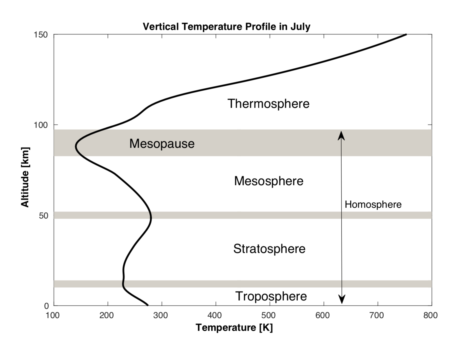
Energy balance is controlled by


Gravity wave
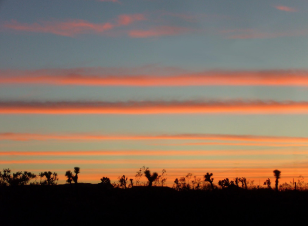
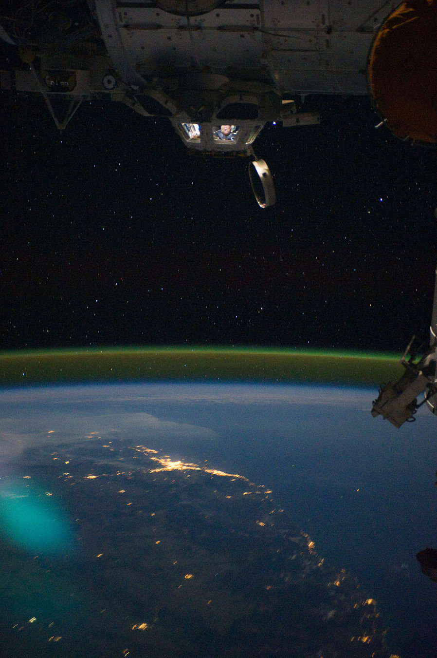
Airglow
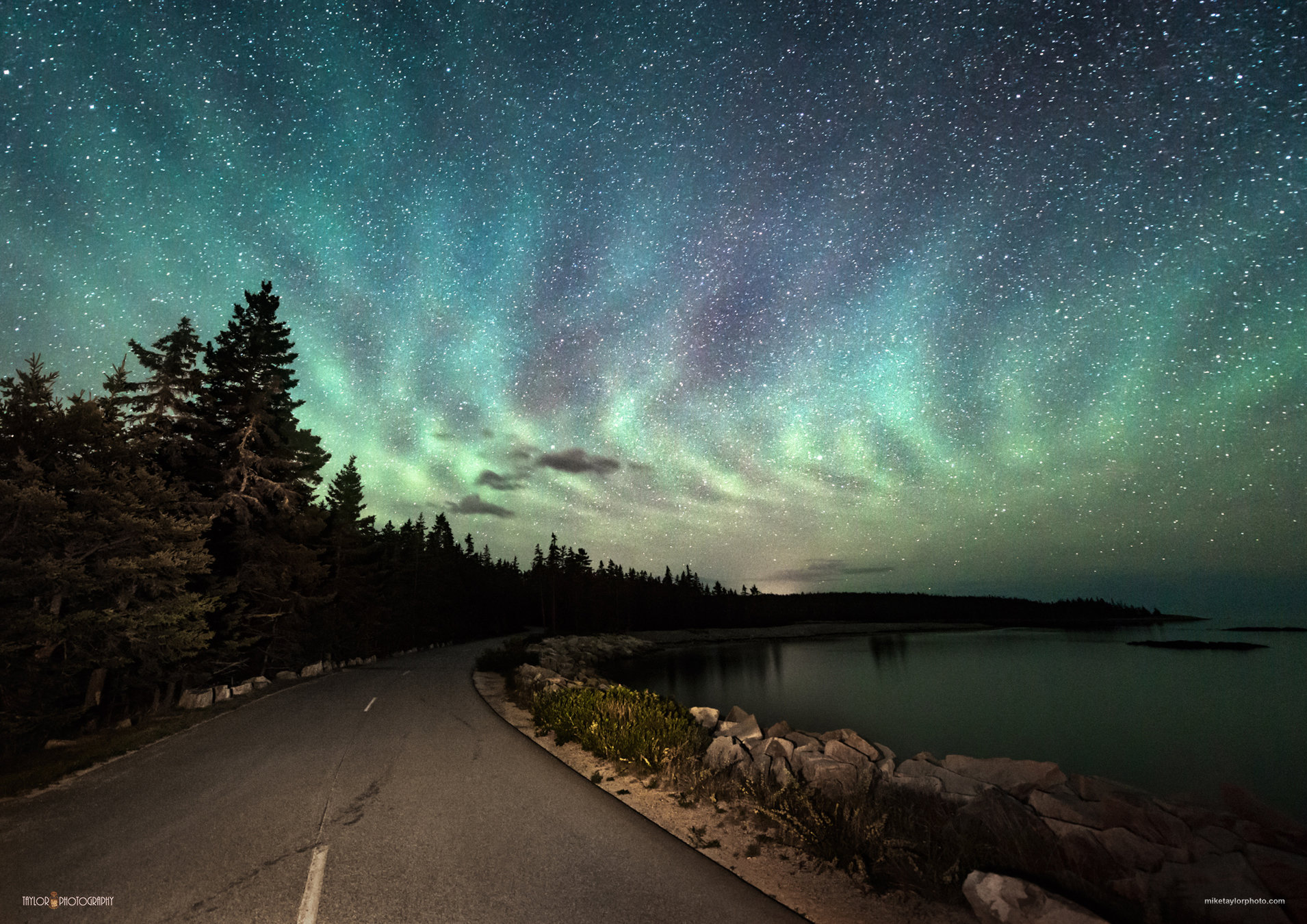
Image from NASA

Image by Mike Taylor and Sonia MacNeil
Odin
SubMillimetre Radiometer (SMR)
Optical Spectrograph and InfraRed Imaging System (OSIRIS)
MATS
2 Ultraviolet Imagers
4 InfraRed Imagers

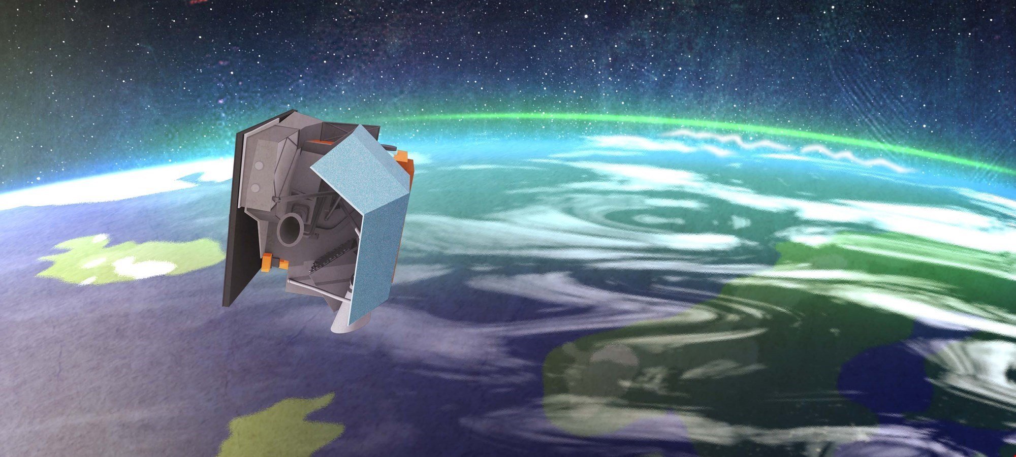
2001~
2020~ ?
- Limb viewing
- Sun-synchronous, near-terminator, polar orbit
- Observes mesosphere
Airglow

Odin-IRI-O2 channel
Observation
N pole
S pole
EQ
EQ
MATS - IR channel
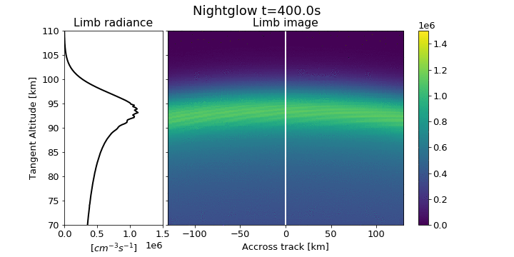
Simulation

Dispersion relation
Q = A \cos(\textcolor{red}{k_x} x + \textcolor{red}{k_y} y + \textcolor{red}{k_z} z + \textcolor{red}{\omega} t)
3D wave
k_x, k_y, k_z, \omega,
stratification
(inside medium)
Doppler relation
\Omega = \omega - \vec{U} \cdot \vec{k}
Intrinsic freq.
Observed freq.
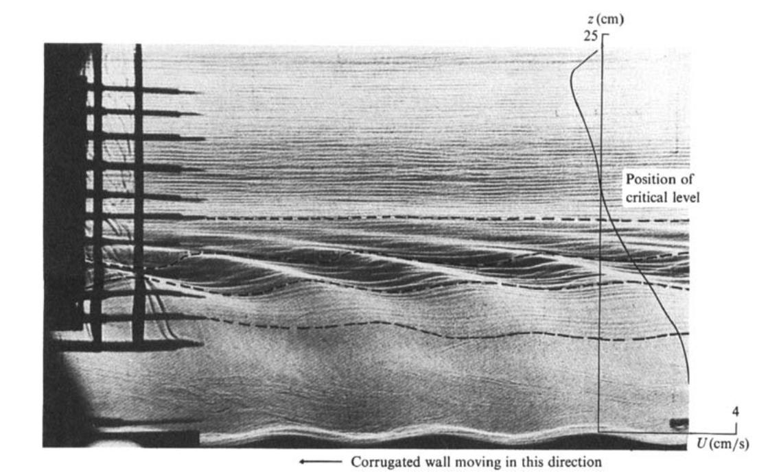
Koop and McGee (1986)
)
)
)
How to sense waves?
- Ground-based vertical profiler (z, t)
- Ground-based sky imager (x, y, t)
- Limb imager (x, (y), z)
How to access intrinsic properties?
make use of
- Doppler relation
- Dispersion relation
Paper 2
Perspectives on
the interpretation of
a gravity wave event
recorded by ground-based lidar
Paper 2
Dörnbrack et al. (2017)
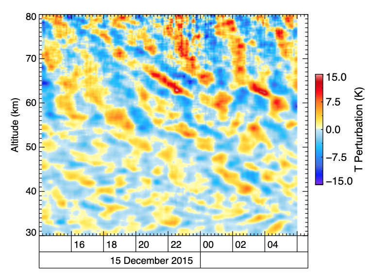
Observed by Rayleigh lidar
Sodankylä, Finland
Wave packet?
Monochromatic
+ Wind change!
Monochromatic
(filtered)
\Omega = \omega - \vec{U} \cdot \vec{k}
Doppler relation
Observed wind
matches
calculated wind
Paper 2
< 0 UTC
> 0 UTC
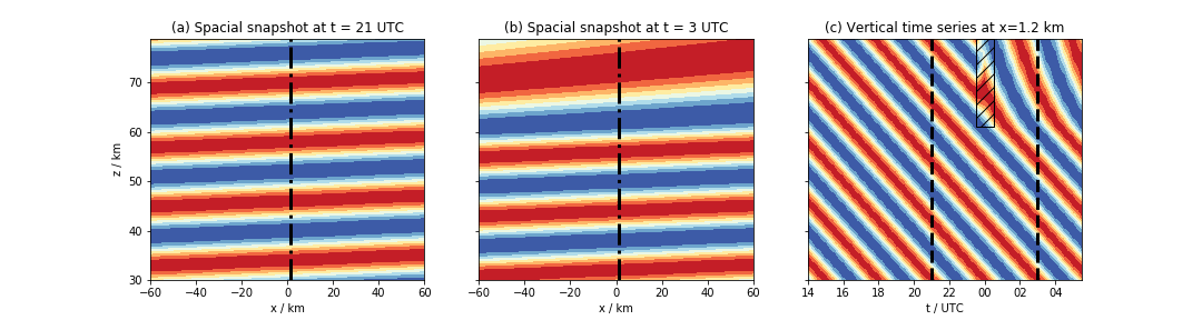
Observed
Simulated
Paper 2
Monochromatic
+ Wind shear change!
(airglow chemistry)
\mathrm{O}(^1D)
\mathrm{O}_3
\mathrm{O}_2(^1\Delta)
\mathrm{O}_2(^1\Sigma)
\mathrm{O}_2
\mathrm{O}
Photochemical model
\mathrm{O}_2(^1\Delta)
\mathrm{O}_2(^1\Sigma)

MATS
Odin-IRI

Paper 1
Retrieval of
daytime mesospheric ozone using OSIRIS observation of
O2 ( ) emission
a^1\Delta_g
Optimal estimation method
a.k.a.
Bayesian statistical approach
Inversion step 1

Limb radiance -> Volume emission rate
\mathbf{y = F (x)}
Limb
Volume
\mathrm{O}_2(^1\Delta)
Paper 1
Result step 1
Paper 1

Volume emission rate
Optimal estimation method
a.k.a.
Bayesian statistical approach
Inversion step 2
\mathbf{y = F (x)}
\mathrm{O}_2(^1\Delta)
Paper 1
\mathrm{O}_3
Non-linear
Levenberg-Marquardt method

Final result
Ozone from Odin compare
Paper 1
Ozone
N pole
S pole
EQ
EQ
- Expansion of the retrievals
- Mesospheric science
- MATS data
Complementary slides
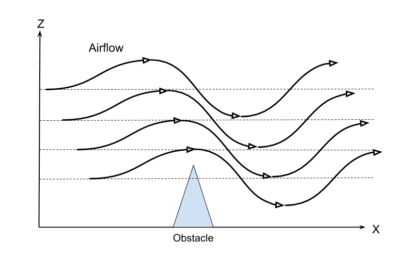
Obstacle effect
Mechanical oscillator
Spontaneous emission
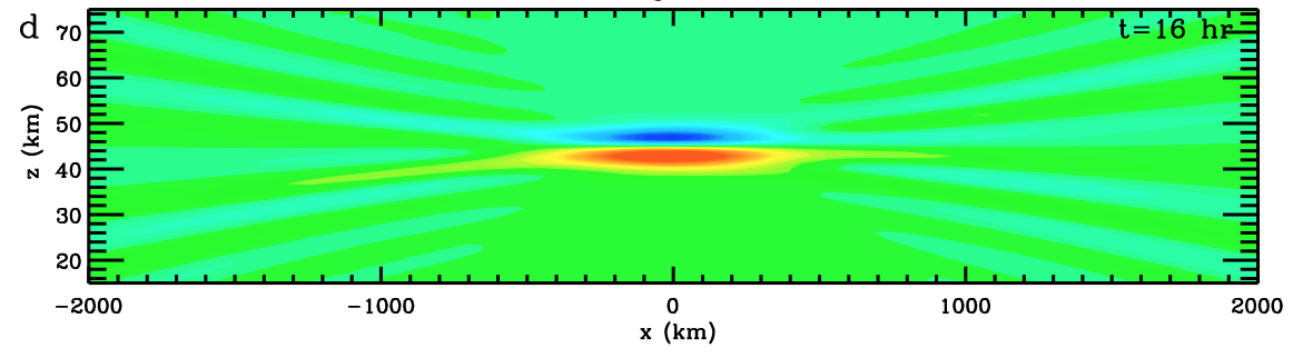
Vadas et. al (2018)
Koop and McGee (1986)

Summer school in Cambridge 2018
Paper 1
Odin- IRI

> 100 pixels vertically
\mathrm{O}_2(^1\Delta)
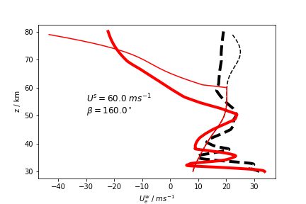
Check horizontal wind (ECMWF + radar)
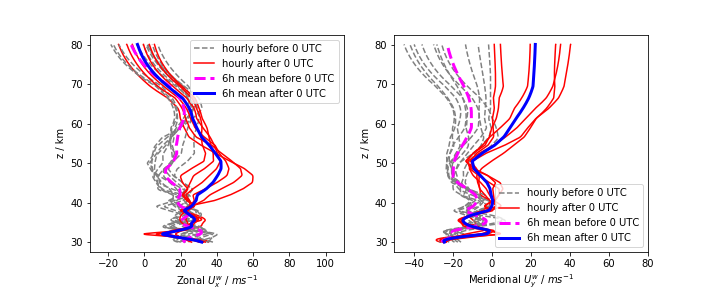
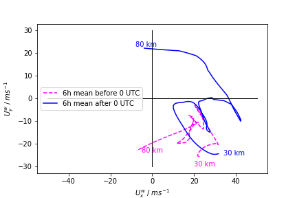
Hodograph
Paper 2


Lic
By ankiki


