Quantum Monte Carlo approaches for strongly correlated systems
Describing correlated electrons
- Lattice models: make assumptions about interactions
- Ab initio descriptions: include general interactions

Strongly correlated electrons



Quantum many-body problem and Monte Carlo

Hilbert space dimension scales exponentially with system size
Quantum Monte Carlo: sample properties without storing full wave functions
Exact simulations \(\rightarrow\) fermion sign problem (exponential decay of signal to noise)

Variational Monte Carlo
Stochastic multireference perturbation theory
Auxiliary field QMC


1902.07690 (2019), 1908.04423 (2020), 2008.06477 (2020)
1909.06935 (2019), 2008.00220 (2020)
2104.06597 (2021)
Outline
- Sampling and the sign problem in AFQMC
- Reducing noise using selected CI wave functions
- Benchmark results
- Jastrow symmetry projected states in VMC
- Auxiliary field QMC
- Variational MC
- Ongoing work
Variational Monte Carlo (VMC)
Strategy:
- Parametrize the wave function: \(|\psi(\mathbf{p})\rangle\), choose initial \(\mathbf{p}\)
- Calculate energy and gradient: Markov chain Monte Carlo
- Optimize: smart gradient descent to change parameters

Ground state minimizes
McMillan (1965)
Symmetry projected mean field states
Symmetry breaking \(\rightarrow\) more variational freedom*
Projection in VMC by restricting random walk to the symmetry sector
* in finite systems
Symmetries: spin, number, complex conjugation, ...
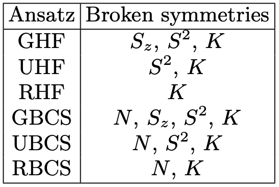
Break symmetries under a projector, to retain good quantum numbers
Mean field state: eigenstate of a quadratic Hamiltonian
Antisymmetrized geminal power (AGP)
Breaking number symmetry
\( F_{p\uparrow,q\downarrow} \rightarrow\) amplitude for the bond between \( p \) and \( q \)
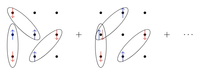
BCS wavefunction in real space
Resonating valence bond state if double occupations are filtered out
H\( _8 \) linear chain (8e, 8o)
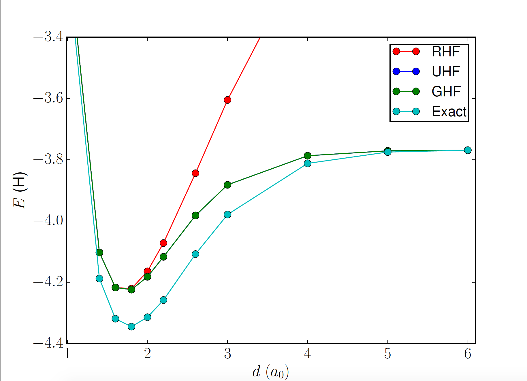
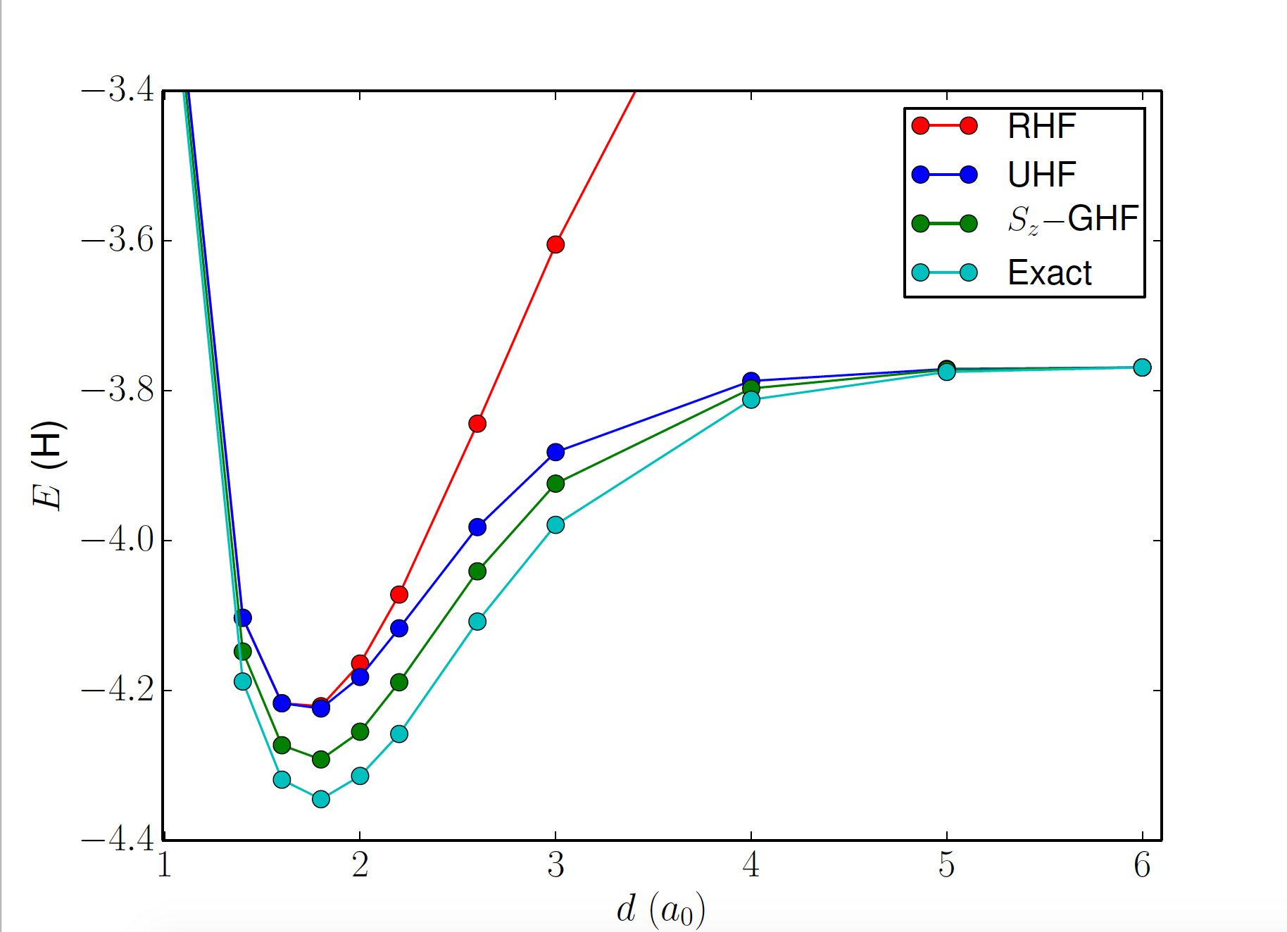
restoring \( S_z \) symmetry
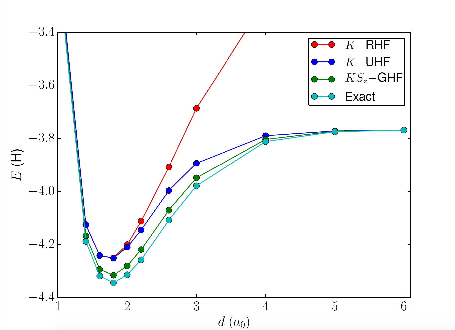
restoring \( S_z \) and \( K \) symmetries
Jastrow factor
counts site occupations and suppresses spurious ionic configurations (double occupations)

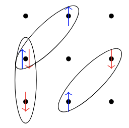


also correlates doublons and holons: important for describing insulators
| d (Bohr) | Exact (DMRG) | Jastrow-KSzPfaffian | Green's function MC |
| 1.6 | -0.5344 | -0.5337 | -0.5342 |
| 1.8 | -0.5408 | -0.5400 | -0.5406 |
| 2.5 | -0.5187 | -0.5180 | -0.5185 |
H\( _{50} \) linear chain (50e, 50o)
| U | Benchmark energy | Jastrow- KSzGHF |
Green's function MC |
| 2 | -1.1962 | -1.1920 | -1.1939 |
| 4 | -0.8620 | -0.8566 | -0.8598 |
| 8 | -0.5237 | -0.5183 | -0.5221 |
2D Hubbard: 98 sites (half filling)
Hartree/particle

Density-density correlation function: 18 site 2D Hubbard model (\(U/t=4\))
Projection QMC
- Better \(|\psi\rangle\) approximates \(|\Psi_0\rangle\), faster the convergence with \(\tau\)
Mixed energy estimator:
Trial states: Selected CI, Jastrow, MPS, ...
- Noise in QMC sampling worsens exponentially with \(\tau\) (sign problem)
Imaginary time propagation
Sampling in AFQMC
Exponentiating \(\hat{H}\): \([\hat{K}, \hat{V}] \neq 0\)
- Exponentiating \(\hat{K}\): orbital transformation
where \(|\phi\rangle\) and \(|\phi'\rangle\) are nonorthogonal determinants.
- Exponentiating \(\hat{V} = \frac{1}{2}\sum_{\gamma} \left(L^{\gamma}_{pr}\hat{a}_p^{\dagger}\hat{a}_r\right)^2\):
\(x_{\gamma}\): auxiliary field
Motta and Zhang (2017), 1711.02242
(Thouless, 1960)
(Stratonovich, 1957)
Sample Gaussian auxiliary fields \(X\), propagate, and measure

The sign problem

Contour shift:
In AFQMC:
Baer, Head-Gordon, Neuhauser (1998)


Selected CI trial state as \(|\psi_l\rangle\)
Zero variance principle: If \(|\psi_l\rangle\) is the exact ground state, then \(N\) and \(D\) are perfectly correlated, \(\langle\psi_0|\hat{H}|\phi_i\rangle = E_0 \langle\psi_0|\phi_i\rangle\), and the energy estimator has zero variance. More accurate \(|\psi_l\rangle\ \rightarrow\ \) higher \(\text{Cov}(N, D)\).

\((\text{H}_2\text{O})_2\), (16e, 80o)
Selected configuration interaction: put the most important configurations in the state using particle-hole excitations and diagonalize
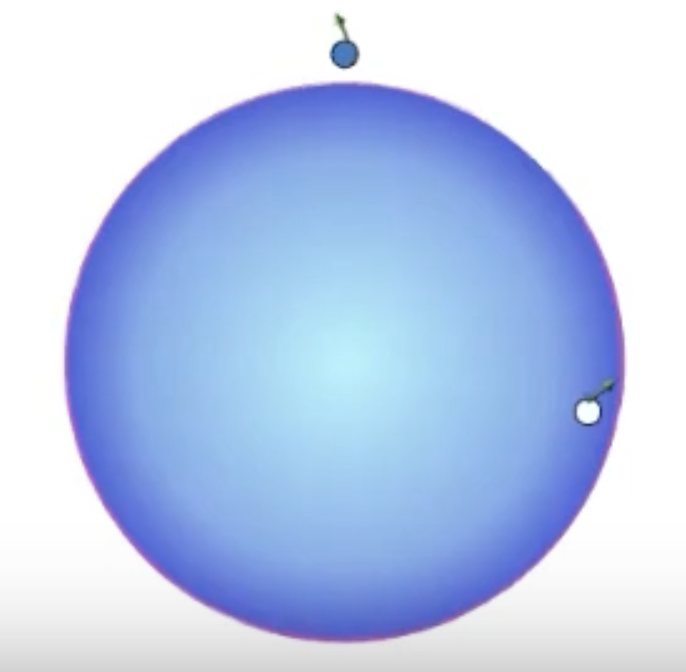
Selected CI local energy algorithm

Generalized Wick's theorem: consider \(|\psi_l\rangle = c_{ptqu}\hat{a}_t^{\dagger}\hat{a}_p\hat{a}_u^{\dagger}\hat{a}_q|\psi_0\rangle\)

\((\text{H}_2\text{O})_2\), (16e, 80o)
\([\text{Cu}_2\text{O}_2]^{2+}\) isomerization


kcal/mol

Phaseless AFQMC

\(\text{H}_{50}\) (50e, 50o)
Gets rid of the sign problem, but has a systematic trial dependent bias
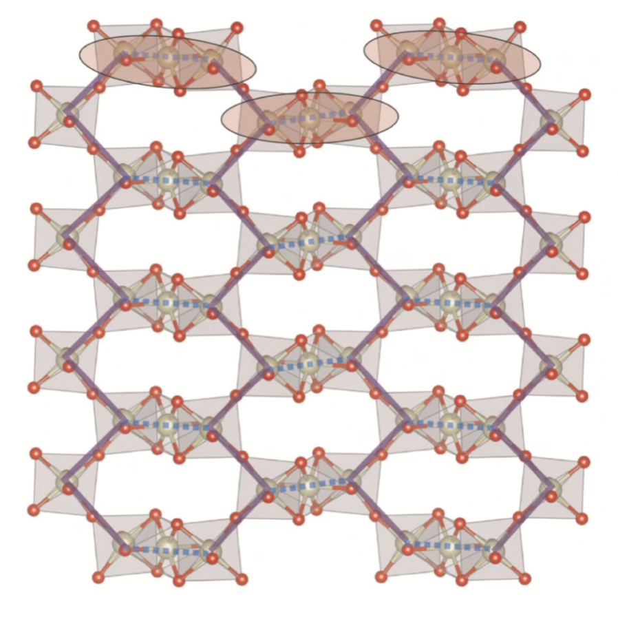
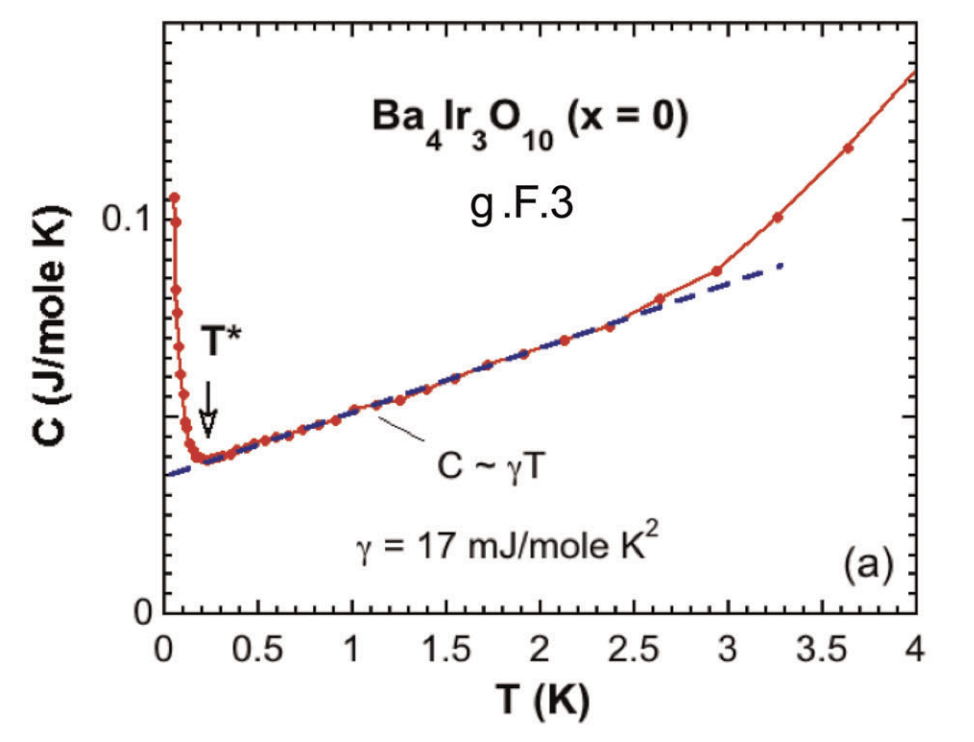
Quantum spin liquid in \(\text{Ba}_4\text{Ir}_3\text{O}_{10}\)?
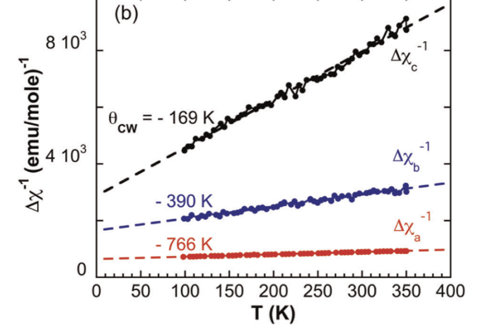

inverse susceptibility
heat capacity
- Insulator with T-linear heat capacity
- Interactions ~ 500 K but orders at 0.2 K
- 2D but not geometrically frustrated
G. Cao, et al. (2020) 1901.04125
Ab initio wave function calculations
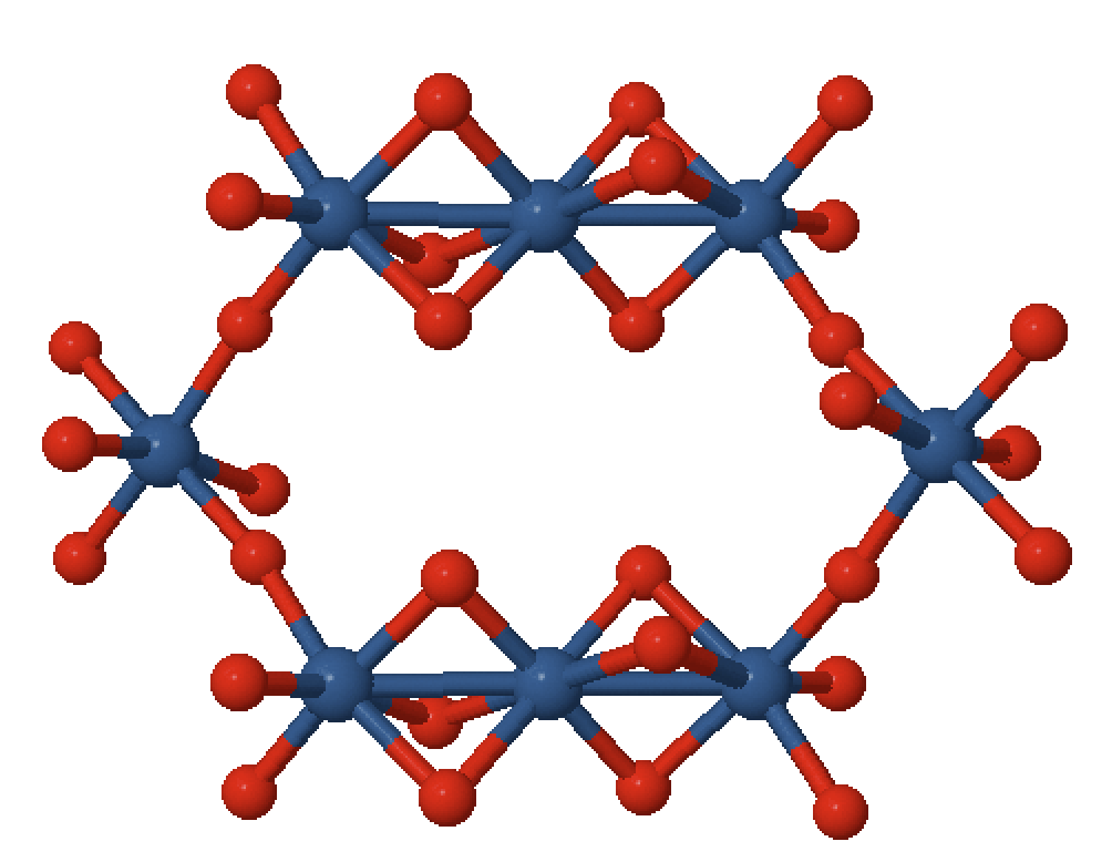
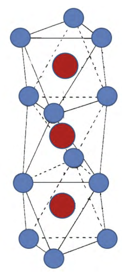
Face shared octahedra
Calculating valence electron wave functions for embedded clusters including all relevant interactions
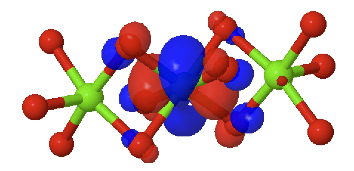
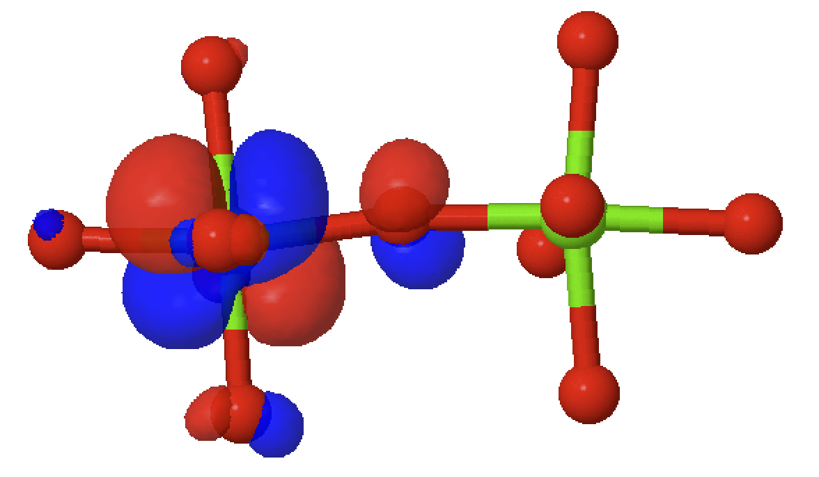
Low lying energy levels:
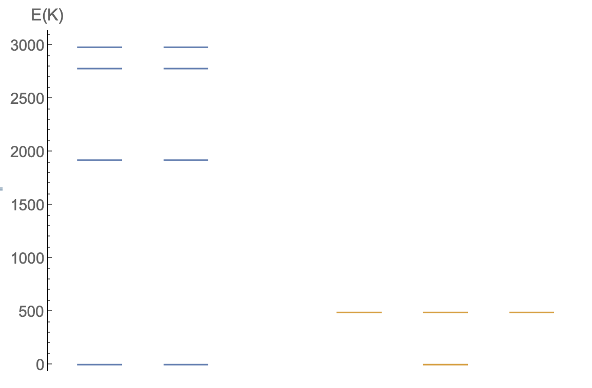
Face shared
Corner shared
Future directions
- Properties and excited states
- Importance sampling and constraints in AFQMC, hybrid MD-MC
- Variational CCSD, other wave functions like MPS, Jastrow in AFQMC
- Spin liquid states in iridates using VMC
Thank you!
afqmc_vmc_1
By Ankit Mahajan
afqmc_vmc_1
- 253


