Stochastic electronic structure theory
Describing correlated electrons
- Lattice models:
- Ab initio descriptions:


The quantum many-body problem and Monte Carlo

Number of configurations increases exponentially with system size
Quantum Monte Carlo: sample properties without storing full wave functions
Exact simulations \(\rightarrow\) fermion sign problem


Variational Monte Carlo
Stochastic multireference perturbation theory
Auxiliary field QMC


Outline
- Sampling and the sign problem in free projection
- Reducing noise using selected CI wave functions
- Phaseless constraint and trial state bias
- Symmetry projected states in VMC
- Auxiliary field QMC
- Variational MC
Free projection AFQMC
- Better \(|\psi_l\rangle\) and \(|\psi_r\rangle\) approximate \(|\Psi_0\rangle\), faster the convergence with \(\tau\)
Mixed energy estimator:
- Numerically exact but noise in QMC sampling worsens exponentially with \(\tau\)
Imaginary time propagation:
Sampling in AFQMC
Exponentiating \(\hat{H}\): \([\hat{K}, \hat{V}]\neq 0\)
- Exponentiating \(\hat{K}\): orbital transformation
where \(|\phi\rangle\) and \(|\phi'\rangle\) are nonorthogonal determinants.
- Exponentiating \(\hat{V} = \frac{1}{2}\sum_{\gamma} \left(L^{\gamma}_{pr}\hat{a}_p^{\dagger}\hat{a}_r\right)^2\):
\(x_{\gamma}\): auxiliary field
(Thouless, 1960)
(Stratonovich, 1957)
Zhang, Krakauer, Reichman, Rubenstein, ...
Sample Gaussian auxiliary fields \(X\), propagate, and measure
Coupled cluster as \(|\psi_r\rangle\): sampling Slater determinants from CCSD
commuting ph excitations \(\rightarrow\) no Trotter error

Benzene (30e, 102o), Hilbert space dimension ~ \(10^{35}\)

The sign problem

Contour shift:
In AFQMC:
Baer, Head-Gordon, Neuhauser (1998)


Zero variance principle
If \(|\psi_l\rangle\) is the exact ground state, then \(N\) and \(D\) are perfectly correlated, \(\langle\psi_0|\hat{H}|\phi_i\rangle = E_0 \langle\psi_0|\phi_i\rangle\), and the energy estimator has zero variance. More accurate \(|\psi_l\rangle\ \rightarrow\ \) higher \(\text{Cov}(N, D)\).
Selected configuration interaction: put the most important configurations in the state using particle-hole excitations and optimize


Benzene (30e, 102o)
Selected CI local energy algorithm

Generalized Wick's theorem: consider \(|\psi_l\rangle = c_{ptqu}\hat{a}_t^{\dagger}\hat{a}_p\hat{a}_u^{\dagger}\hat{a}_q|\psi_0\rangle\)

Benzene (30e, 102o)
\([\text{Cu}_2\text{O}_2]^{2+}\) isomerization

\(\Delta E = E(\text{bis}) - E(\text{peroxo})\)
| Method | |
| DFT (UBLYP) | 36.0 |
| DFT (UB3LYP) | 52.9 |
| DFT (UMPW1K) | 74.0 |
| CCSD(T) | 30.6 |
| CR-CCSD(TQ) | 33.8 |
| DMRG-CT | 27.1 |
| ph-AFQMC (NOCI) | 32.1 |
| fp-AFQMC | 24.1(6) |
kcal/mol
(32e, 108o)
Phaseless AFQMC
- Bias depends on the trial state used
- There is a trade-off between bias and variance
- Phaseless constraint elminates the sign problem at the expense of a bias
\(\text{H}_{50}\) (50e, 50o)


Ni
Excited states of conjugated systems

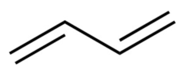
Butadiene: (22e, 142o)
Nickel porphyrin: (122e, 406o)
| Method | ||
| NEVPT2 | 6.72 | 6.74 |
| CCSD | 6.31 | 7.08 |
| AFQMC / sCI | 6.50(5) | 6.67(5) |
| Exact* | 6.2 | 6.5 |
eV
| Method | |
| CASSCF (4e, 4o) | 3.8 |
| CCSD | 2.55 |
| AFQMC / sCI (50k) | 3.0(1) |
| AFQMC / sCI (100k) | 2.8(1) |
| Experiment | 2.3-2.4 |
eV
Other properties
| Species | Exact | CCSD | ph-AFQMC |
| 0.986 | 0.991 | 0.985(2) | |
| 0.990 | 0.992 | 0.986(2) | |
| CO | 0.090 | 0.099 | 0.086(3) |
- Can be evaluated as derivatives of energy
- Derivatives can be calculated just as efficiently as energy (automatic differentiation)
a.u.
Small molecule dipole moment calculations:
NH\(_3\)
H\(_2\)O
Outline
- Sampling and the sign problem in free projection
- Reducing noise using selected CI wave functions
- Phaseless constraint and trial state bias
- Symmetry projected states in VMC
- Auxiliary field QMC
- Variational MC
Variational Monte Carlo (VMC)
Strategy:
- Parametrize the wave function: \(|\psi(\mathbf{p})\rangle\), choose initial \(\mathbf{p}\)
- Calculate energy and gradient: Markov chain Monte Carlo
- Optimize: smart gradient descent to change parameters

Ground state minimizes
McMillan (1965)
Symmetry projection in VMC
Symmetry breaking \(\rightarrow\) more variational freedom
Break the symmetry under a projector, to retain good quantum numbers
Symmetries: spin, number, complex conjugation, ...
Example: complex conjugation in \(\text{H}_2\) near dissociation


Imada, Sorella, Neuscamman, ...

Density-density correlation function: 18 site 2D Hubbard model (\(U/t=4\))
| d (Bohr) | Exact (DMRG) | Jastrow-SzPfaffian | Jastrow-KSzPfaffian |
| 1.6 | -0.5344 | -0.5327(2) | -0.5337(2) |
| 1.8 | -0.5408 | -0.5389(2) | -0.5400(2) |
| 2.5 | -0.5187 | -0.5167(2) | -0.5180(2) |
H\( _{50} \) linear chain (50e, 50o)
Hartree/particle
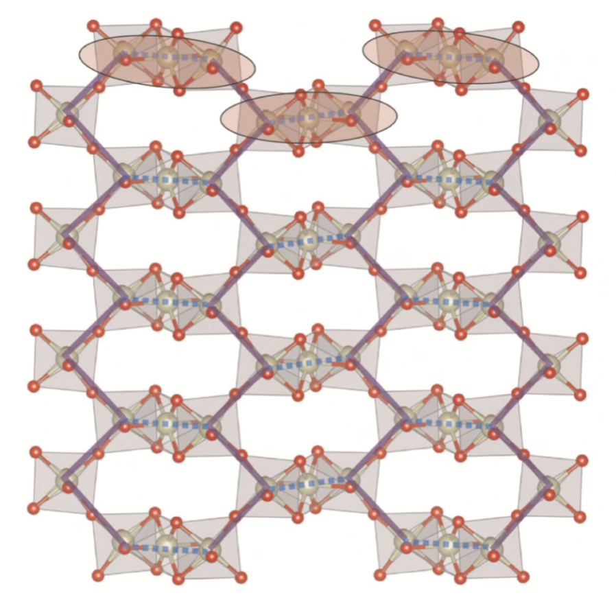
Quantum spin liquid in \(\text{Ba}_4\text{Ir}_3\text{O}_{10}\)?

- Insulator with T-linear heat capacity
- Interactions ~ 500 K but orders at 0.2 K
- Not geometrically frustrated
G. Cao, et al. (2020) 1901.04125

Possible in \(\text{Ba}_4\text{Ir}_3\text{O}_{10}\): \(U(1)\) QSL with \(|\psi_0\rangle\) a metallic free fermion state
Gutzwiller projection with VMC:
Savary, Balents (2016)
Summary and outlook
- Combining ideas from QMC and quantum chemistry is a useful approach
- Scalability and parallelizability mean they can be used for studying much larger correlated systems
- QMC techniques are very flexible, so can be employed in a variety of problems
- Possible future directions:
- AFQMC: excited states, dynamics, solids,...
- VMC: neural network states, spin liquids,...
Thank you to:
- The committee
- Sandeep and the Sharma group
- Friends and family
- Funding from NSF and CU Boulder
- Teachers, mentors, collaborators
defense
By Ankit Mahajan
defense
- 317


