Jastrow Multi-Slater Wave Functions
Localized vs. itinerant electons

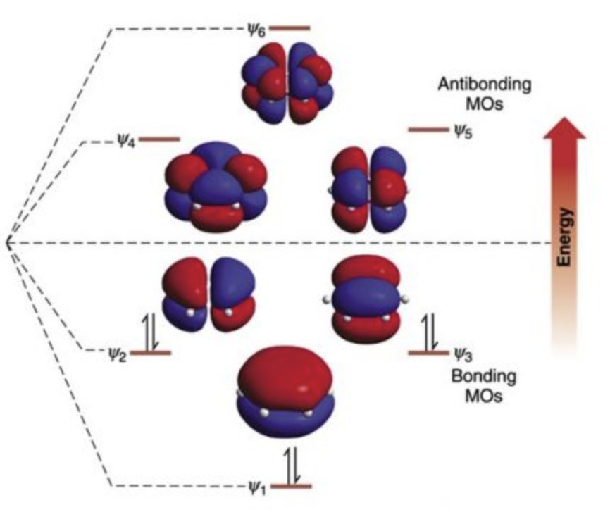
| H\(_{30}\) | Benzene | |
| HCI | -16.203 (13m dets) | -230.556 (3m dets) |
| JS | -16.219 | -230.505 |
penalizes fluctuations
energetic excitations
Jastrow
Slater
Combine the two!: Jastrow multi-Slater
- it systematically improves Jastrow Slater
- could be used in a large class of systems as a black box method
- many interesting phenomena occur at the interface of local-itinerant regimes
We think this is a winner because:
How shall we implement this?
- using VMC, of course!
- not trivial to do this efficiently
Quick VMC redux
Energy of a wave function is calculated as

walker
local energy
\(H\) generates excitations
single: \(O(N^2)\)
double: \(O(N^4)\)!

Calculating overlaps
unlike \(H\), \(J\) does not generate excitations
For a Jastrow Slater wave function
Now for overlap with \(|\phi_0\rangle\), consider:
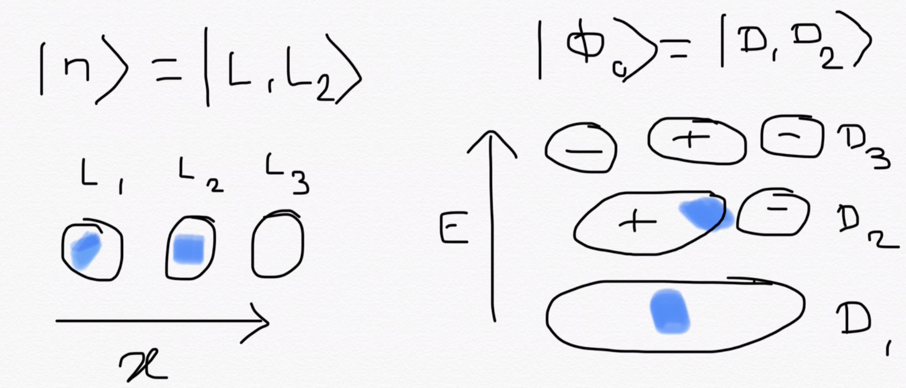
Overlaps are determinants
Roughly, \(\langle L_1L_2|D_1D_2\rangle\) = Amplitude\((|L_1L_2\rangle\rightarrow|D_1D_2\rangle)\)
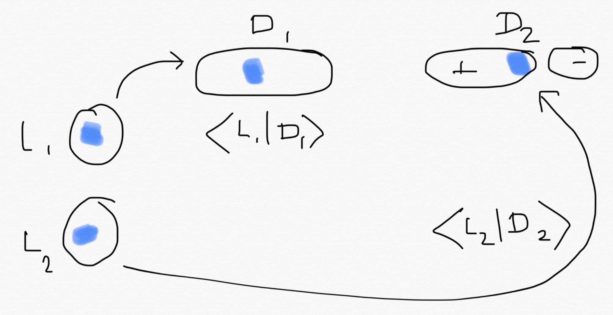
Two ways to accomplish this process
\(L_1\rightarrow D_1\) and \(L_2\rightarrow D_2\): \( \langle L_1|D_1\rangle \times \langle L_2|D_2\rangle\)
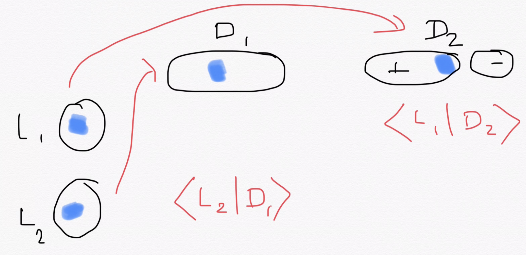
\(L_1\rightarrow D_2\) and \(L_2\rightarrow D_1\): \( \langle L_1|D_2\rangle \times \langle L_2|D_1\rangle\)
or
fermion antisymmetry (exchange)
Properties of determinants

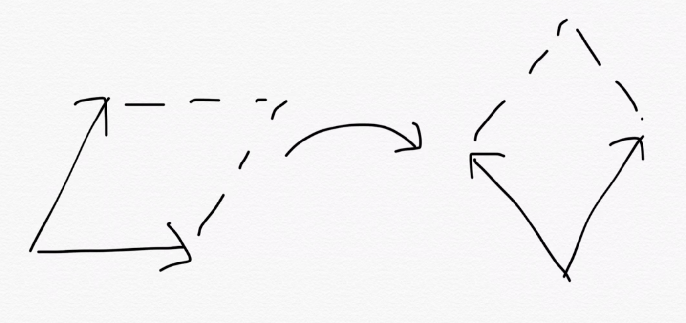
Determinants are volumes
(up to sign)
Some things are easy to prove using this geometric viewpoint:
volumes don't change under rotation
\(= \det\left(\hat{a},\hat{b}\right)\)
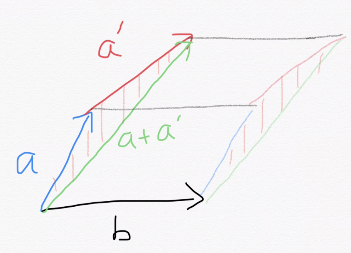
(HF invariance to unitary rotations)
linearity
Calculating determinants is expensive!
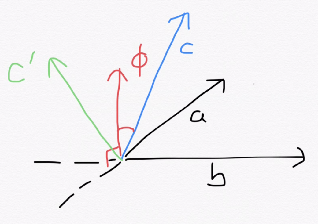
Let's build up the volume progressively:
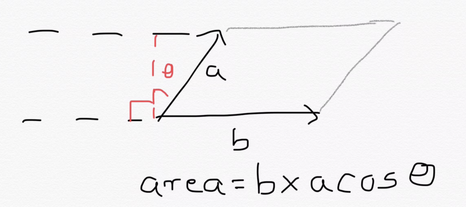
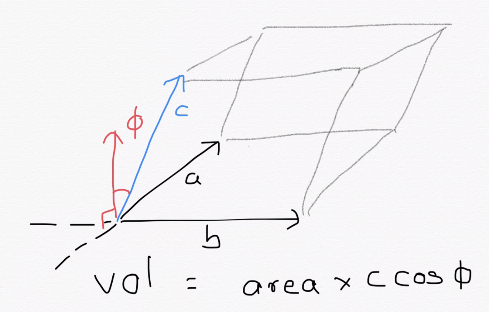
and so on...
We need the direction orthogonal to the span in the previous iteration to sweep the volume in that direction. This process has total cost \(O(N^3)\).
Observation: the orthogonal direction is given by the corresponding column of the inverse matrix!
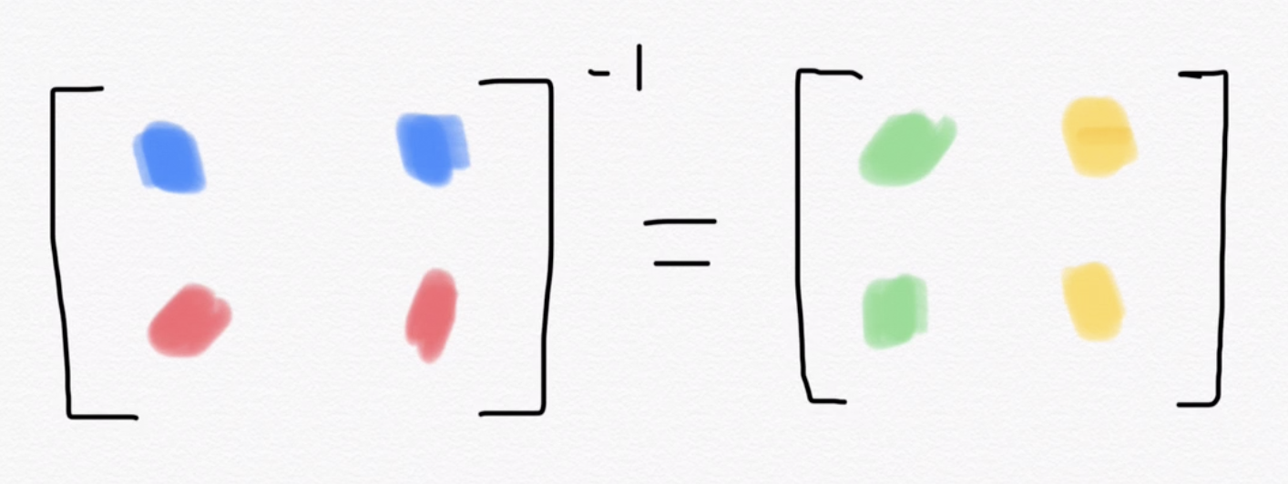
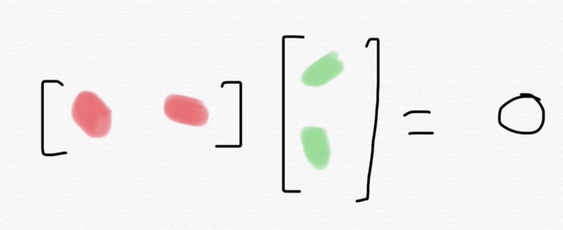
A naive approach to local energy calculation would cost \(O(N^3\times N^4)\) (there are \(O(N^4)\) Hamiltonian excitations).
Paying attention to what's changing
Suppose \(|n\rangle = |L_1L_2\rangle\), and \(|m\rangle = a_3^{\dagger}a_2|L_1L_3\rangle\) is an excitation generated by the Hamiltonian.
Note that only a row in the determinant changed. We need to generate a lot of excitations from \(|n\rangle\), but their overlap determinants differ from that of \(|n\rangle\) by at most two rows.
So we don't need to repeat the work of calculating the volume of the unchanged vectors or orthogonal directions.
3rd column of the inverse
Matrix determinant lemma
Local energy picture
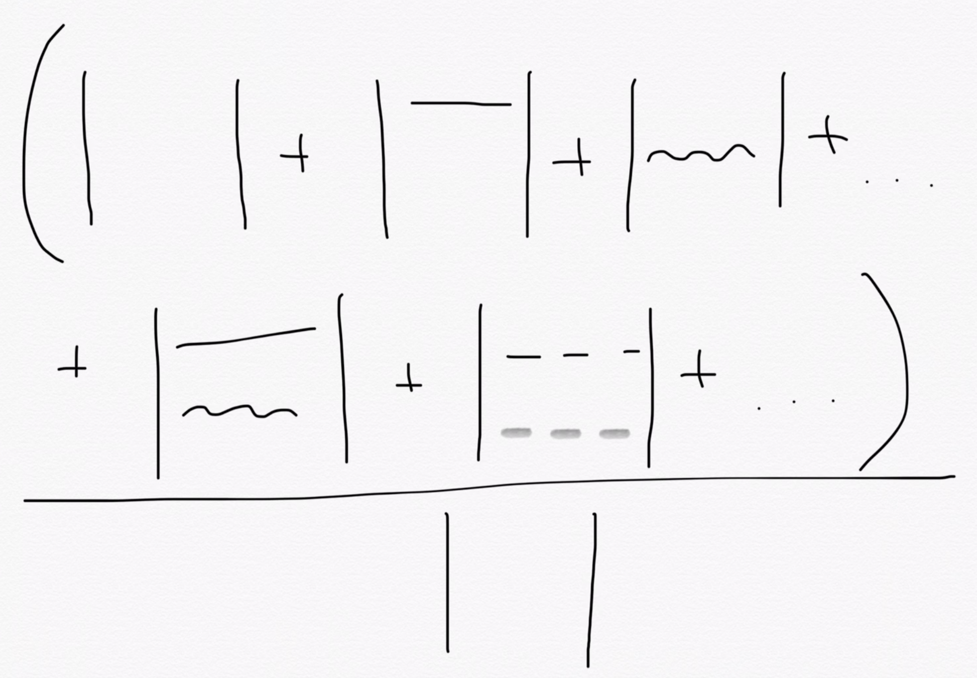
Leading cost: \(O(N^4)\)
\(O(N^4)\) terms
Multi-Slater wave function overlap
excitations of delocalized orbitals
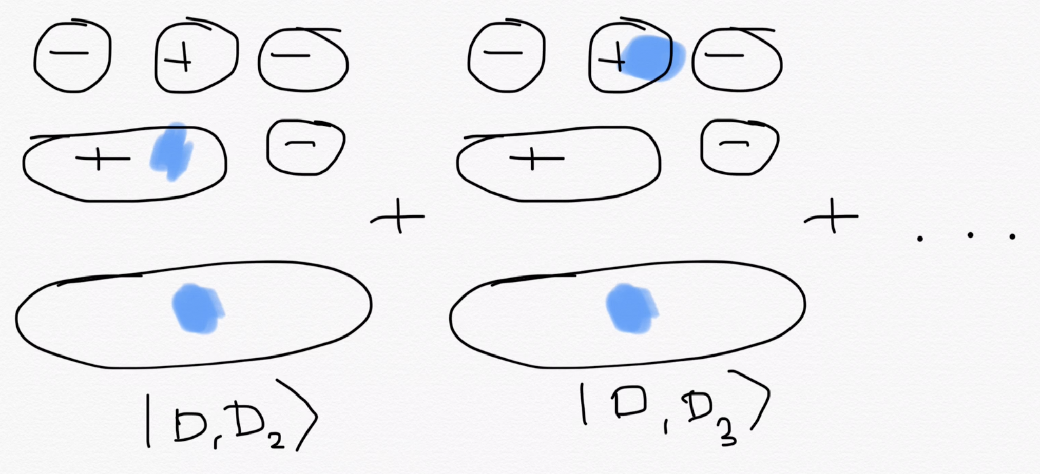
Overlaps of individual delocalized configurations with local configuration \(|n\rangle = |L_1L_2\rangle\) are
Note that only the second column is different. The same logic as before applies to column changes as well! The overlap cost is \(O(N_e)\).

Local energy of multi-Slater
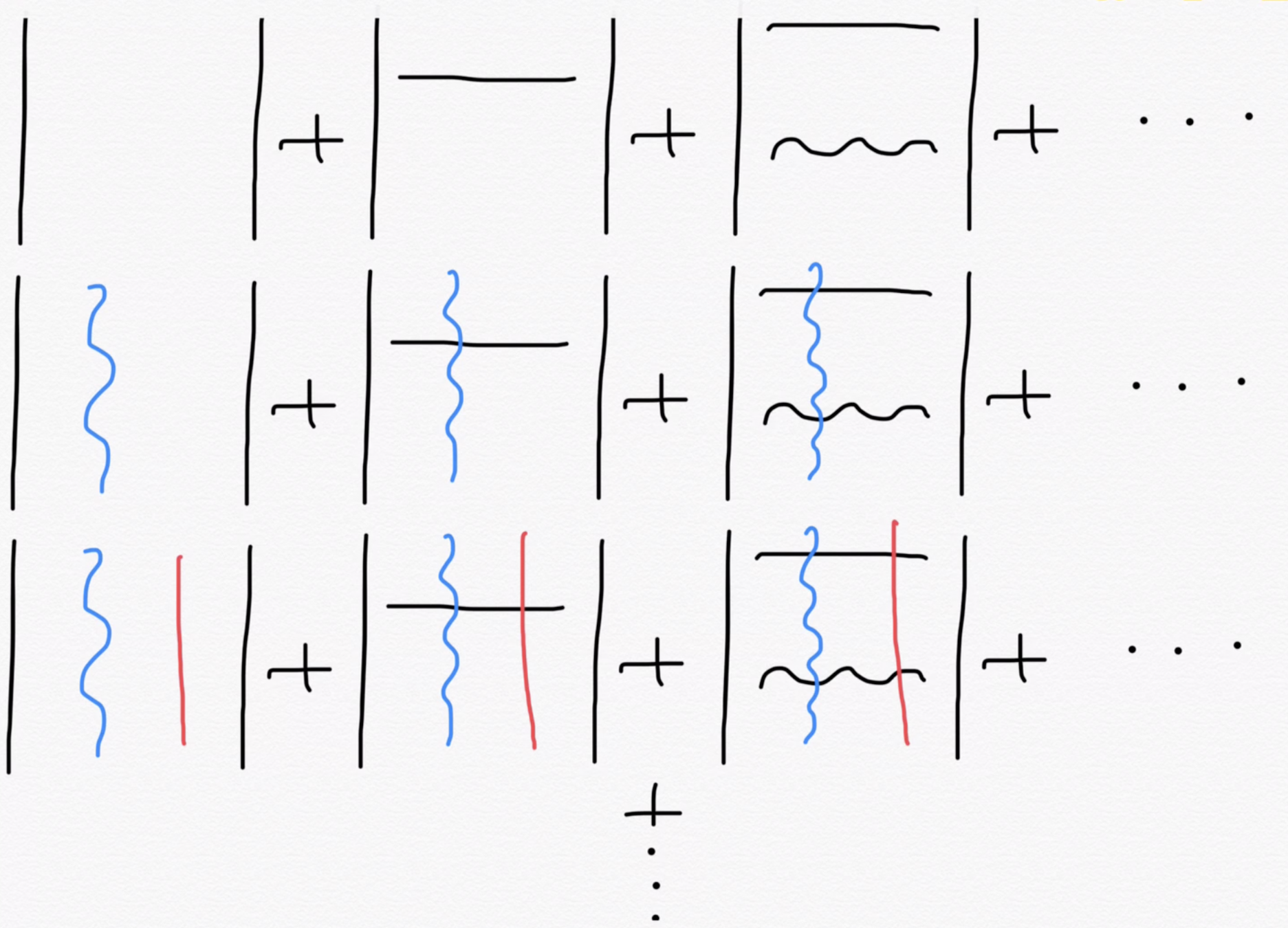
A naive calculation would cost \(O(N_eN^4)\), which is not feasible when \(N_e\) is in thousands or more. Can we do better?
row replacements due to \(H\) excitations
column replacements due to wave function \(\hat{E}_i\) excitations
Efficient local energy calculation
The basic idea again is to pay attention to what's changing in these determinants and store useful intermediates.
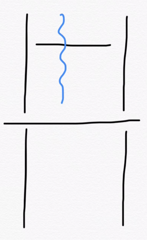
row replacement
column replacement
cross element
In the term that deals with the cross element, we can sum over \(i\) and \(a\) once, and store this as an intermediate. Then for any \(j\) and \(b\) the local energy can be calculated in constant time!
Indices \(i\) and \(a\) correspond to \(H\) excitations, while \(j\) and \(b\) to wave function excitations. To calculate local energy we sum over \(i\) and \(a\)
For single excitations, this trick reduces cost to \(O(N_e) + O(N^4)\).
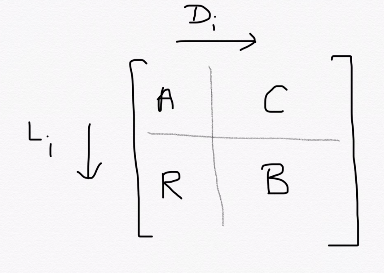
parts of the coeffs matrix
Double excitations are trickier
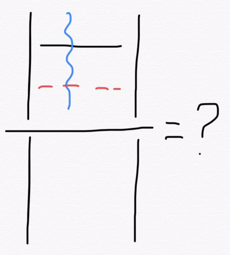
- One possibility is to consider double excitations as combinations of single excitations and proceed as before. This has cost \(O(N_eN^2)\), which is not ideal.
- In principle, we know/can derive a formula for this ratio and see if we can store other intermediates to bring down this cost. Work in progress!
- Another approach I did not talk about involves looking at excitations as derivatives. May be useful as well.

jastrow_multislater
By Ankit Mahajan
jastrow_multislater
- 311


