


Andreas Park PRO
Professor of Finance at UofT
Andreas Park
Traditional Markets
What is Market Microstructure?
Broker
Exchange
Internalizer
Wholeseller
Darkpool
Venue
Settlement
Traditional Institutions
Investors
Trading Arrangements
central limit order book
complexity
price impact of trades
anonymity
price discovery
centralized auction
bilateral
negotiation
Request
for Quote
open
outcry
Who trades?
Key question for liquidity provision
Seminal papers
What's there first? Orders or Liquidity?
Seminal papers
Basics of liquidity provision under value uncertainty
Questions:
every model has some form of structure like
\[\text{trading income (fees, spreads, etc)} +\underbrace{\text{what I sold it for}-\text{value of net position}}_{\text{positional gain/loss}} \ge \text{outside option} \]
Example 1: Grossman/Miller
Example 2: Kyle or Glosten-Milgrom
Example 3: Limit order market (a la Glosten 1994)
Crypto vs TradFi Markets
Key Differences Defi vs TradiFi
Broker
Exchange
Internalizer
Wholeseller
Darkpool
Venue
Settlement
Investor
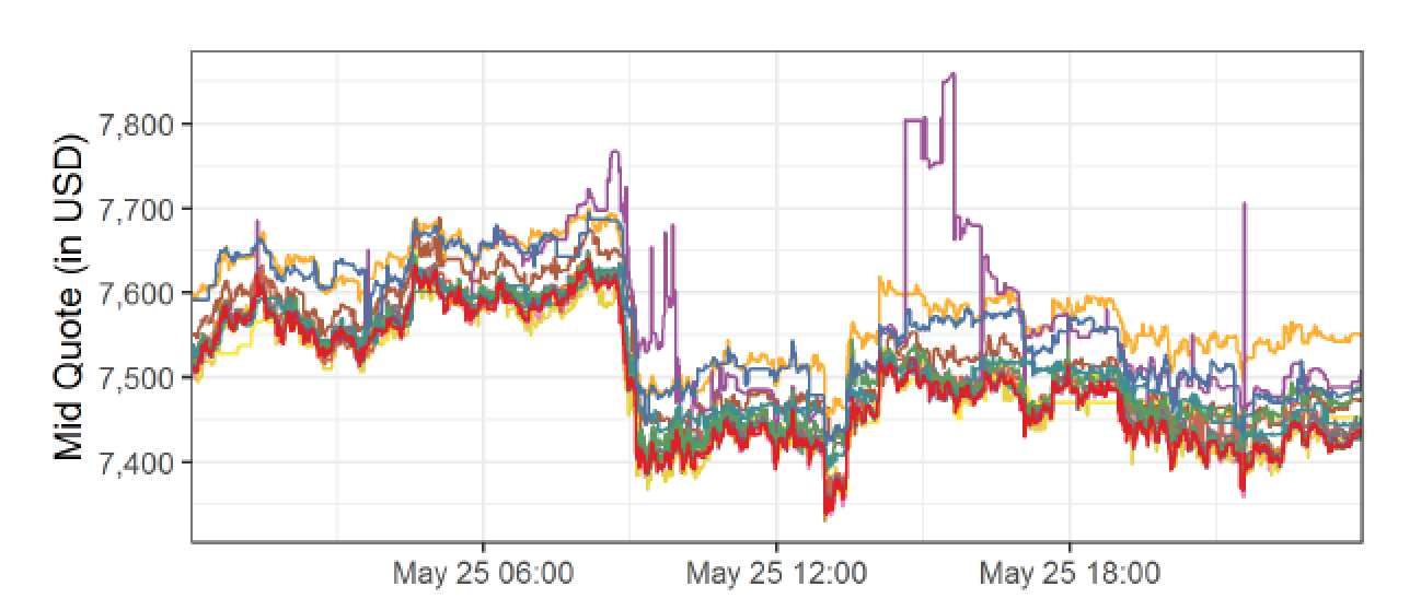
Centralized Trading
BTC/USD
ask: 7,600
bid: 7,550
BTC/USD
ask: 7,500
bid: 7,450
buy BTC
sell BTC
move BTC to Kraken
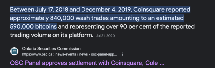
Crypto Wash Trading, Lin William Cong, Xi Li, Ke Tang, Yang Yang
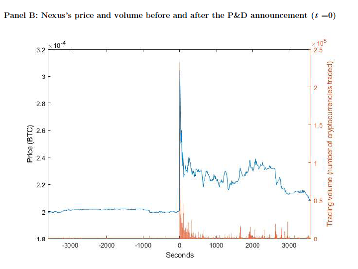
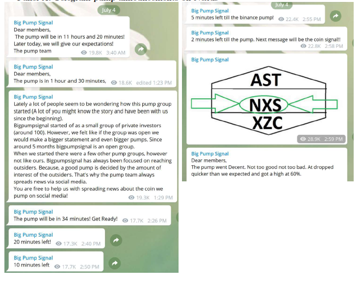
What is pump and dump?
arranged via Telegram Channels
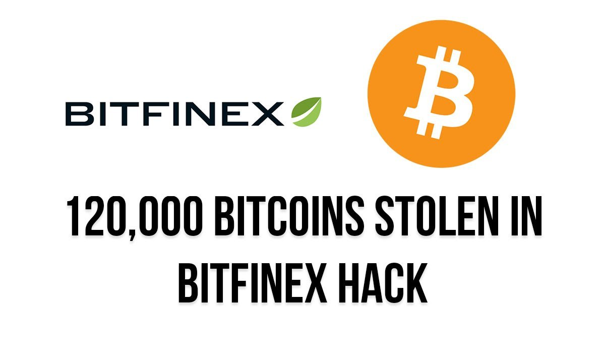
August 2016
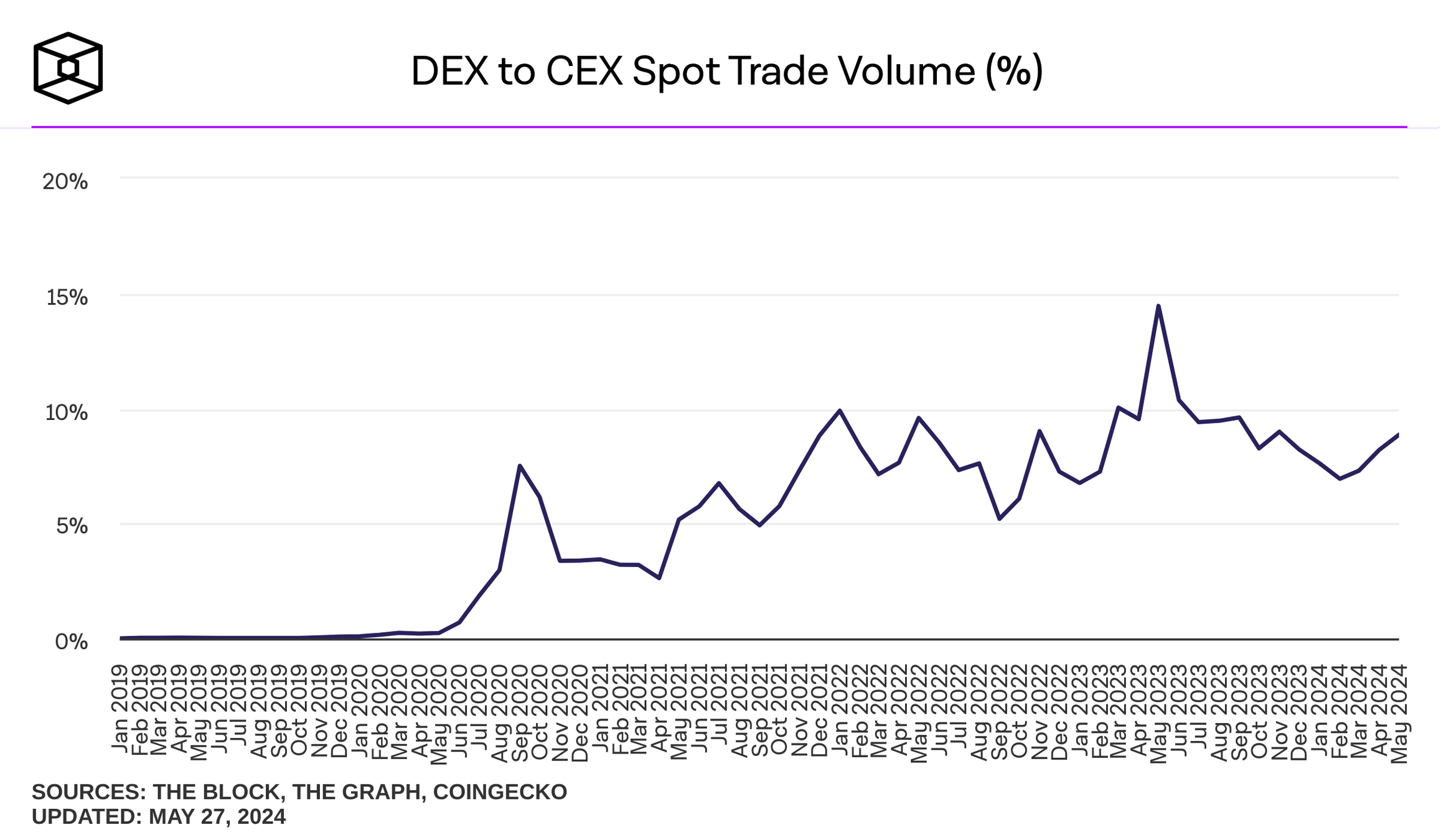
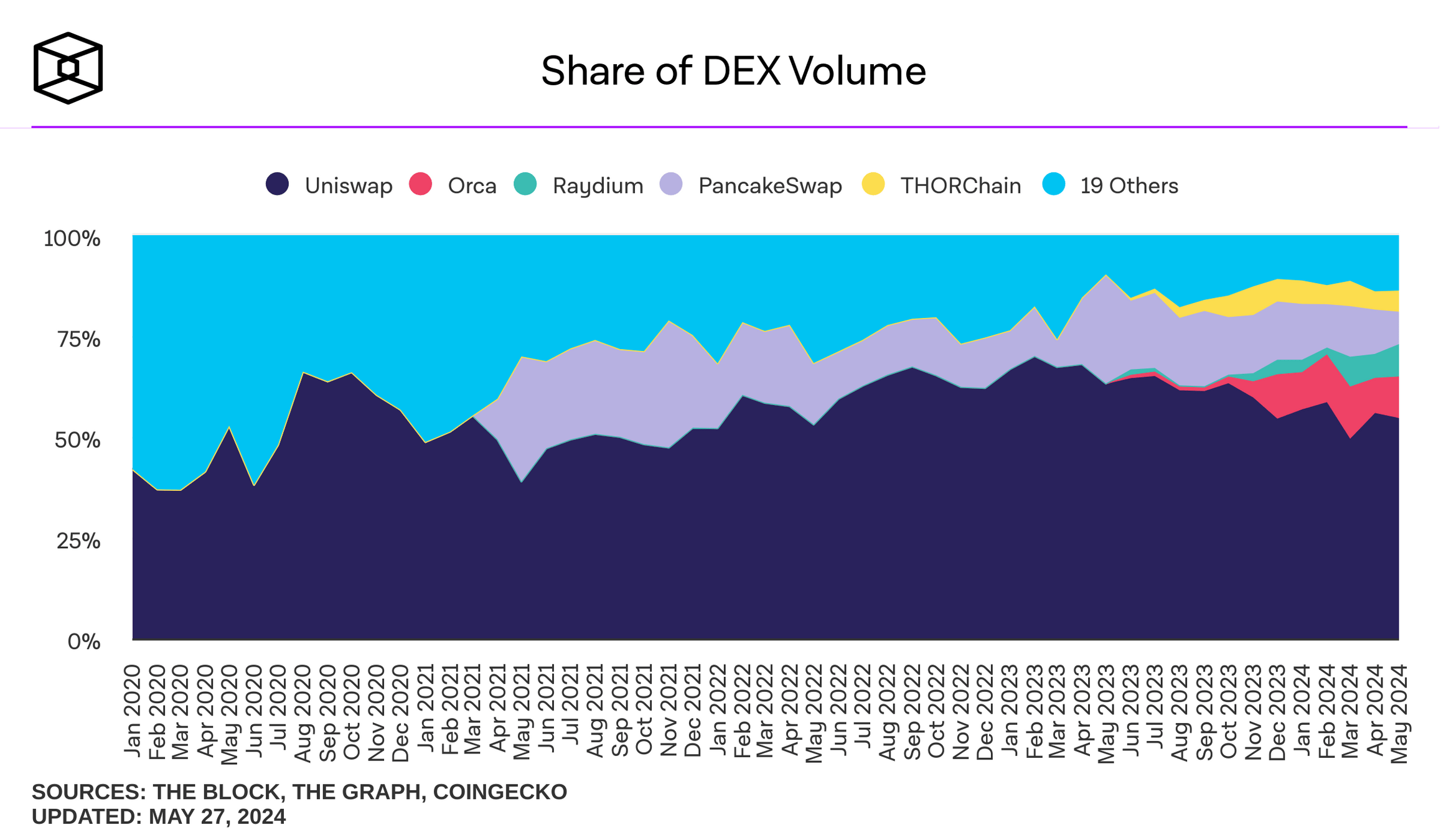
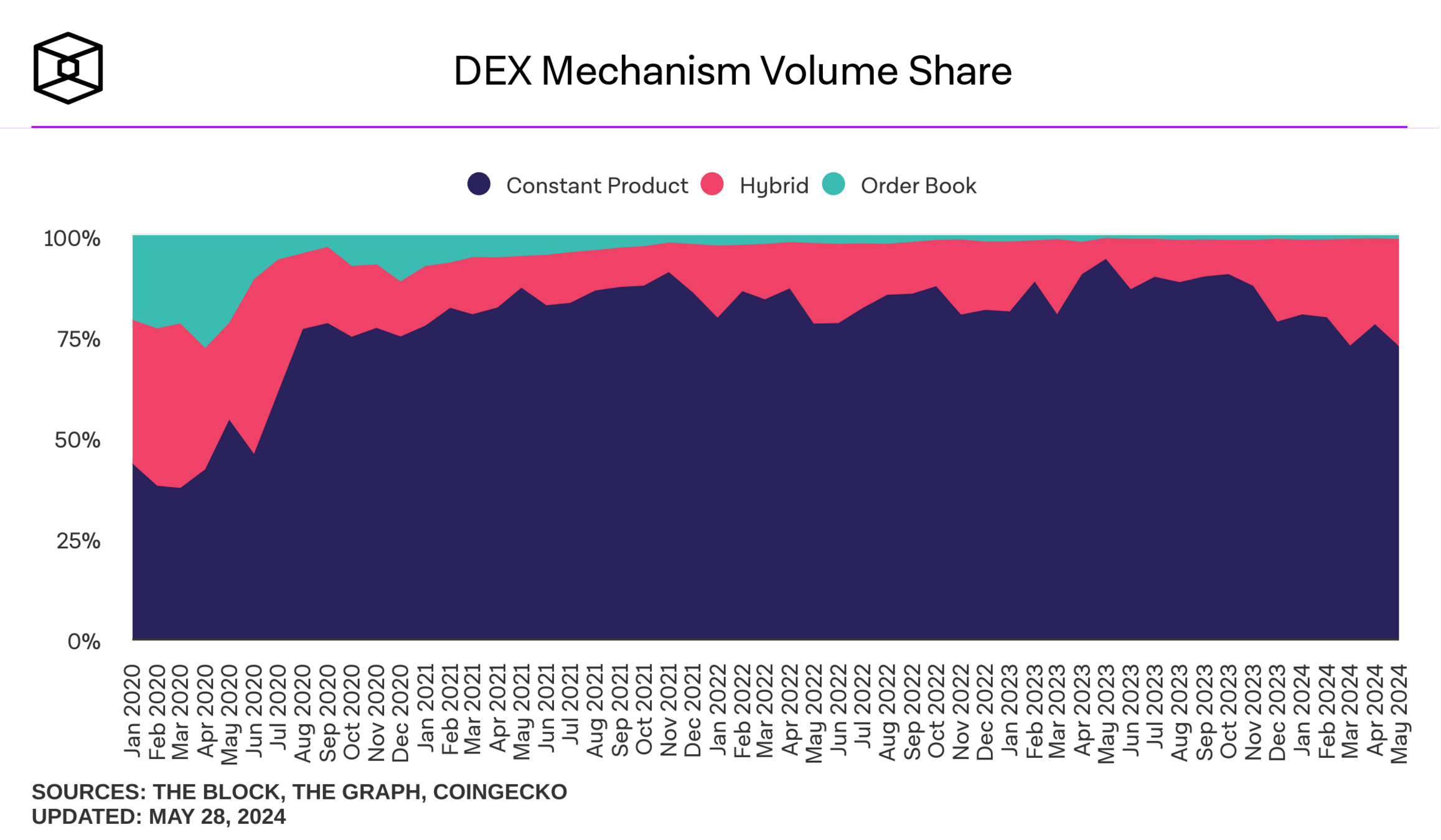
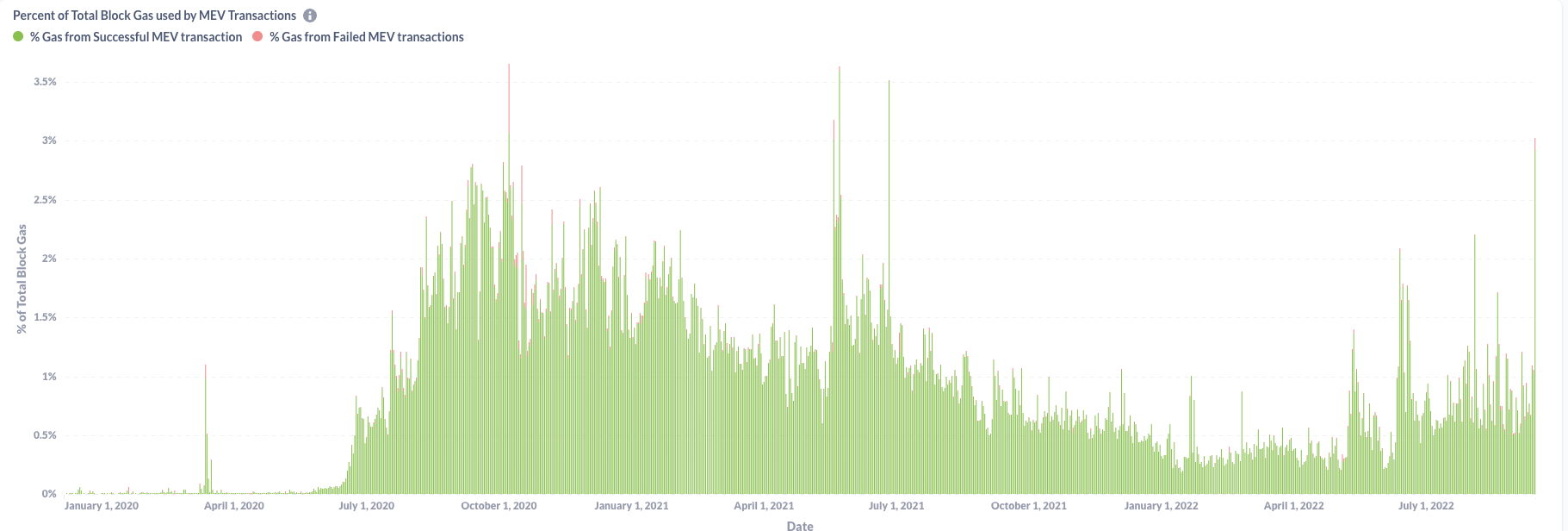
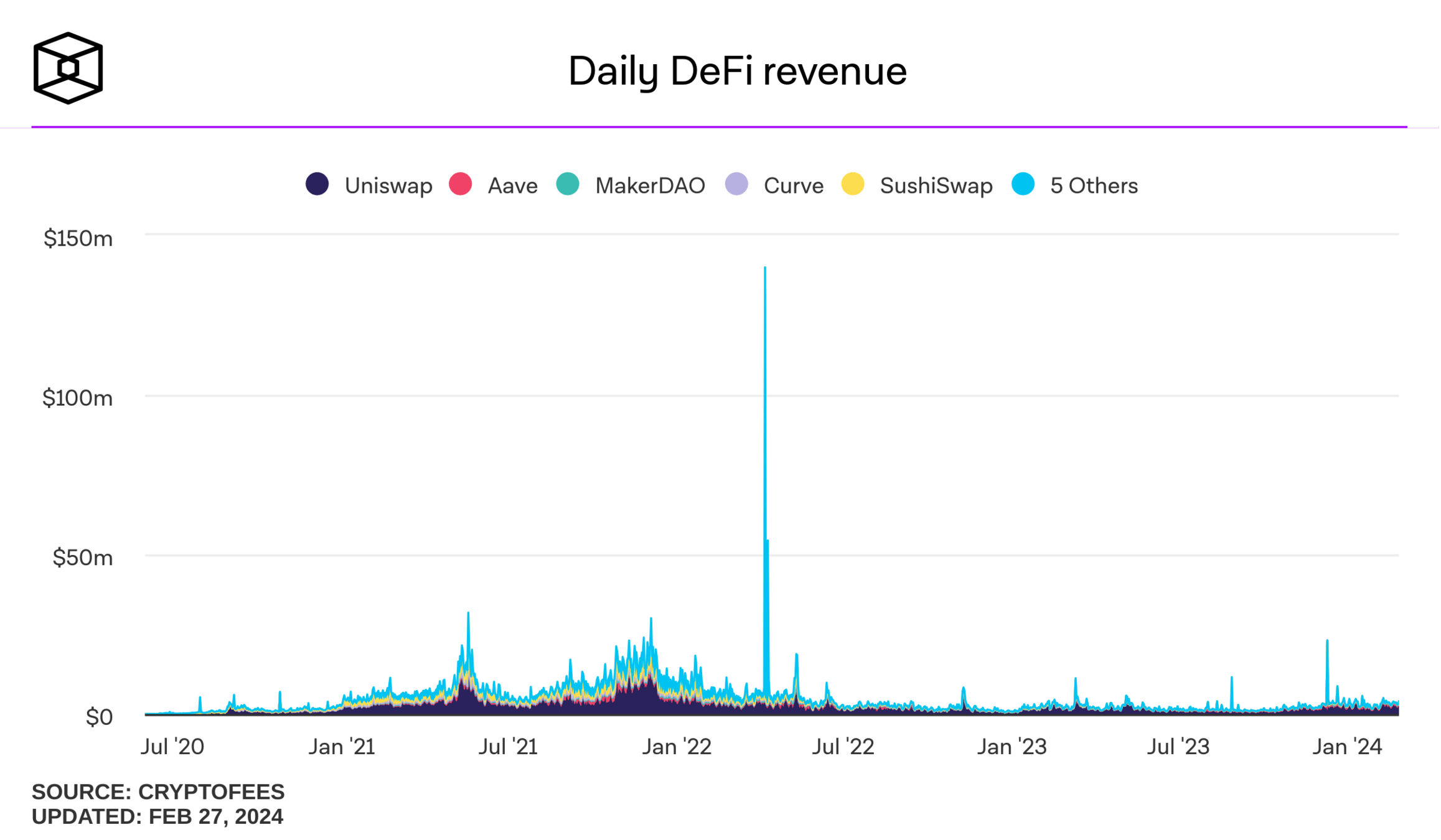
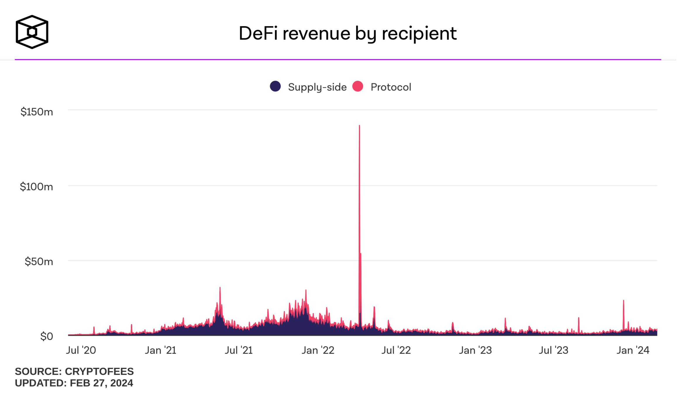
Decentralized Trading
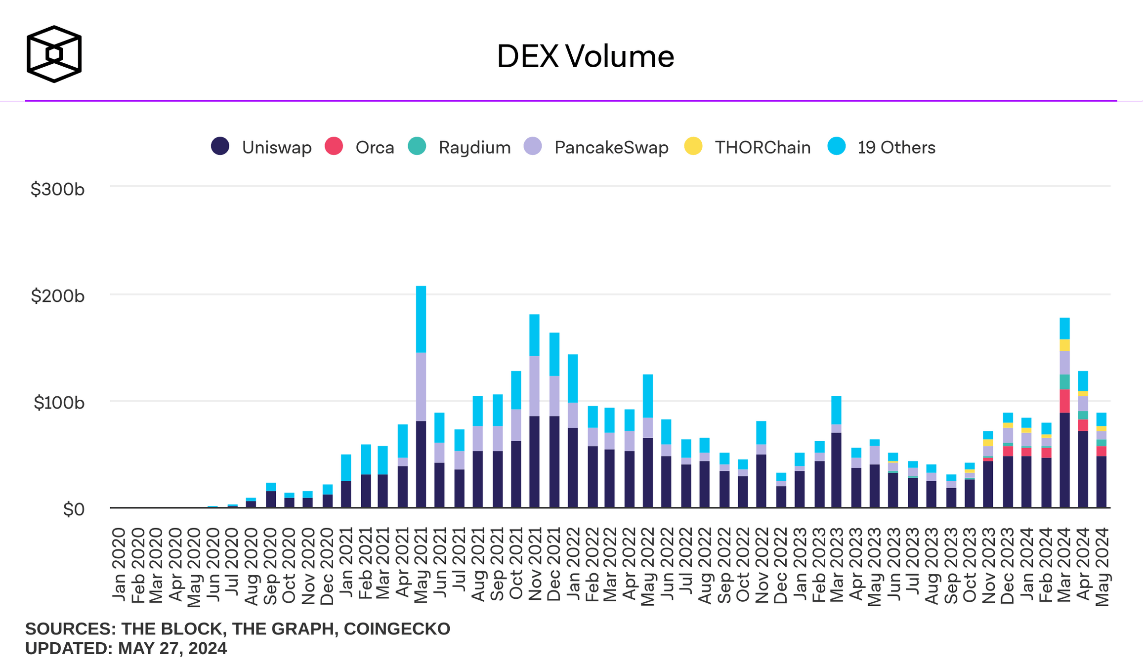
where do I find these plots? theblock.co/data/
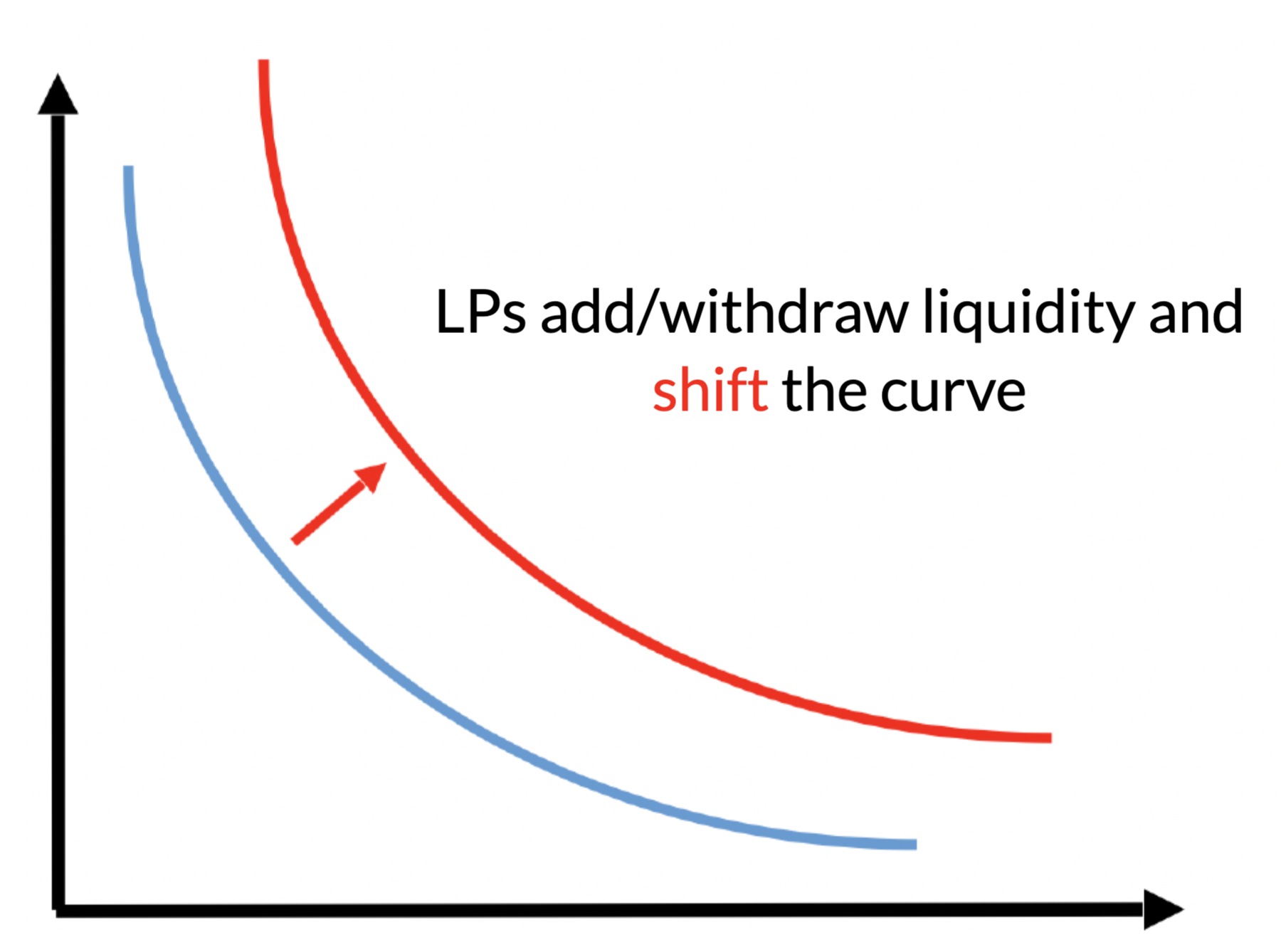
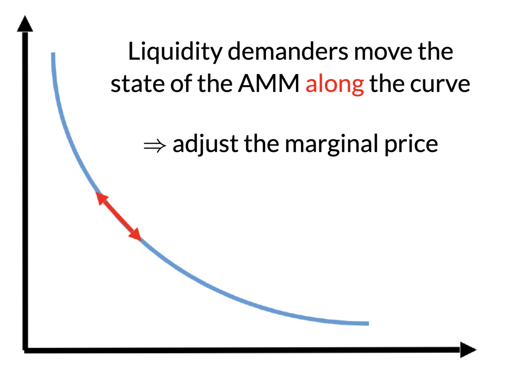
Liquidity providers
Liquidity demander
Liquidity Pool
AMM pricing is mechanical:
No effect on the marginal price
| limit order book | periodic auctions | AMM | |
|---|---|---|---|
| continuous trading |
|||
| price discovery with orders | |||
| risk sharing |
|||
| passive liquidity provision | |||
| price continuity |
|||
| continuous liquidity | |||
| sniping prevented |
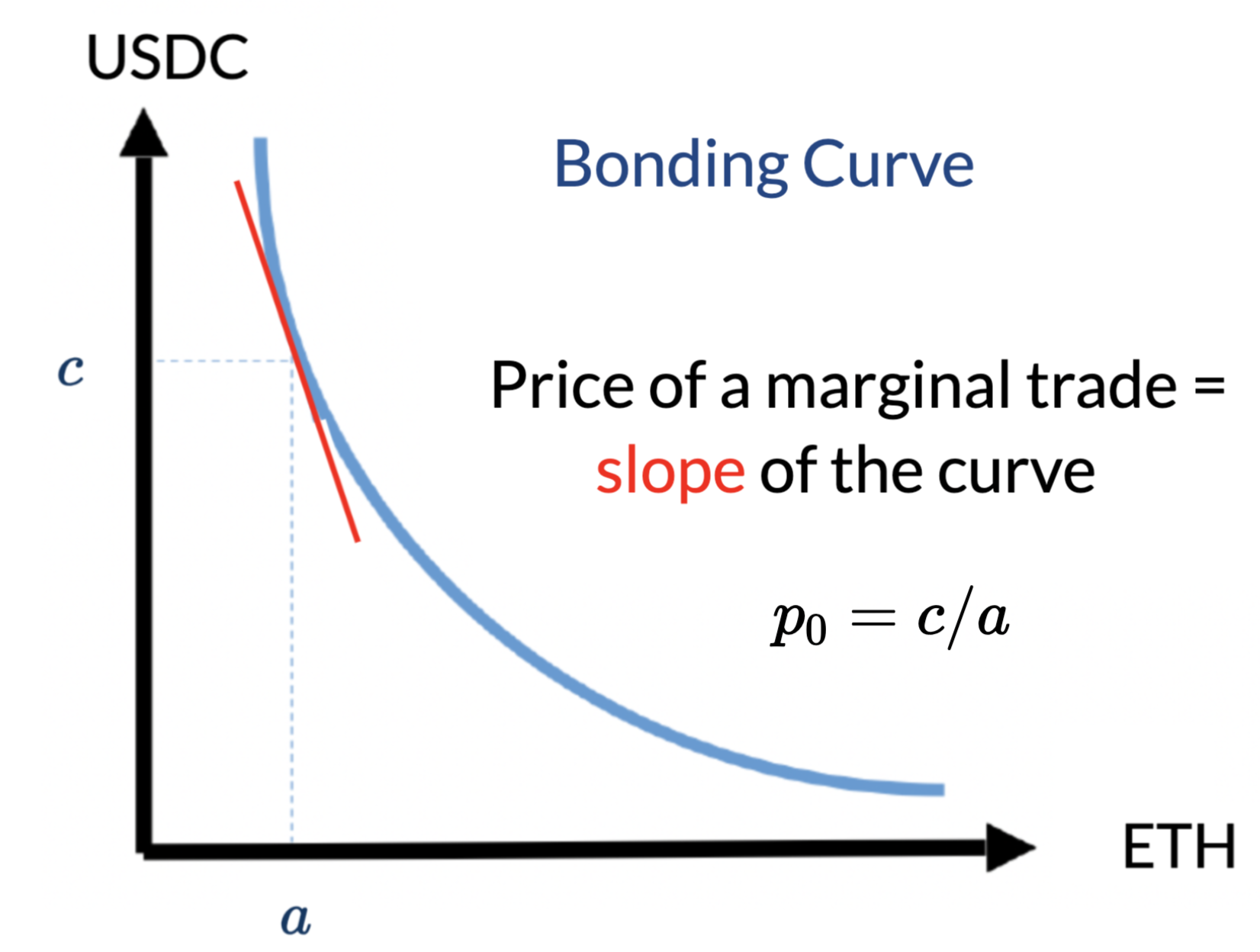
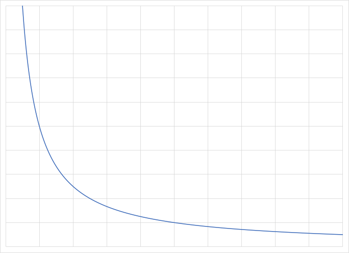
AMM Theory: The Price Function
Basic Requirements
What does an AMM need?
quantity
price
\(q\)
\(p^m(q)\)
\(\Delta c(q)(Q)=p(q)^m\times q\)
Traditional pricing: auctions/open outcry/RFQ: uniform price
idea: cost of \(q=\) price\(\times\) quantity
Some Pricing Rules from Traditional Markets: Uniform Price
\(q=2\)
\(\Delta c(q)= q\times p^m(q)=2\times 15.5\)
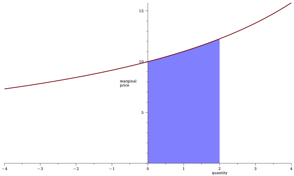
Main pricing rule in stock exchanges: limit order book
quantity
price
\(q\)
\(p^m(q)\)
\(\Delta c(q)=\int_0^qp^m(s)~ds\)
Some Pricing Rules from Traditional Markets: Limit Order Book
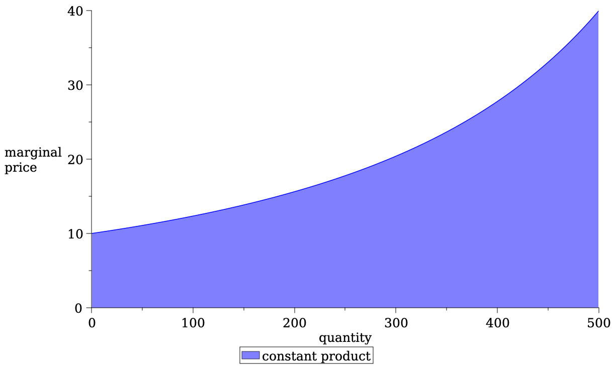
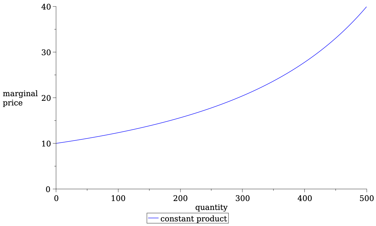
Most Common Pricing Rule in DeFi: Constant Product
Most Common Pricing Rule in DeFi: Constant Product
Insight: AMM pricing function is the same as a limit order book when we require
Some insights on pricing functions
The Pricing Function
Liquidity Supply and Demand in an Automated Market Maker
Liquidity providers: positional losses
Buy and hold
Provided liquidity
in the pool
Two views
Basics of Liquidity Provision
\[\underbrace{F \int DV \mu(DV) }_{\text{fees earned on}\atop \text{balanced flow}}+\int_0^\infty\underbrace{(\Delta c(q^*)-q^*p_t(R)}_{\text{adverse selection loss} \atop \text{when the return is {\it R}}} +\underbrace{F \cdot \Delta c(q^*))}_{\text{fees earned}\atop \text{from arbitrageurs}}~\phi(R)dR \ge 0.\]
\(q^* \) is what arbitrageurs trade to move the price to reflect \(R\)
Basic idea of liquidity provision: earn more on balanced flow than what you lose on price movement
\[\text{fee income} +\underbrace{\text{what I sold it for}-\text{value of net position}}_{\text{adverse selection loss}} \ge \text{cost of capital} \]
in AMMs:
protocol fee
in tradFi: bid-ask spread
Theory Literature on AMM
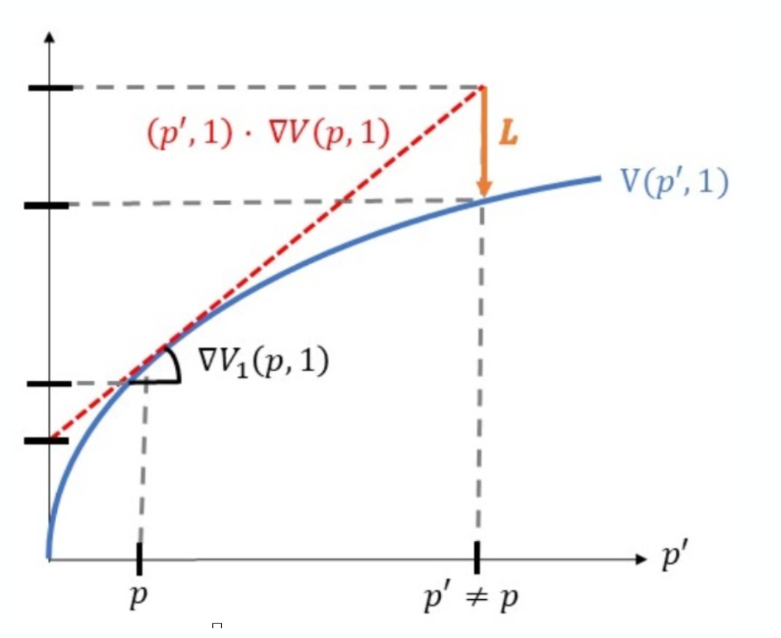
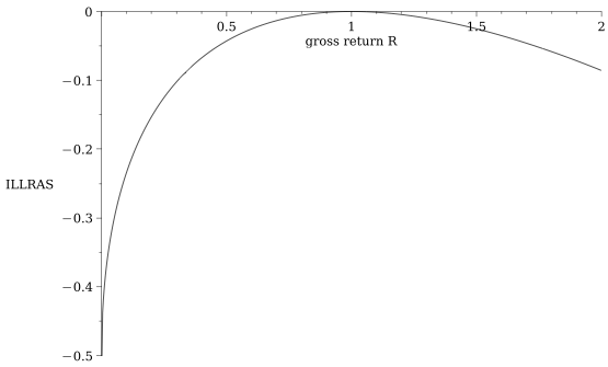
Sidebar: we can quantify how much a PASSIVE LP loses when the price moves by \(R\)
for orientation:
\[\frac{\text{adverse selection loss when the return is \(R\)}}{\text{initial deposit}}=\sqrt{R}-\frac{1}{2}(R+1)\]
see Barbon & Ranaldo (2022)
Liquidity Demander's Decision & (optimal) AMM Fees
Result:
competitive liq provision\(\to\) there exists an optimal (min trading costs) fee \(>0\)
Similar to Lehar&Parlour (2023) and Hasbrouck, Riviera, Saleh (2023)
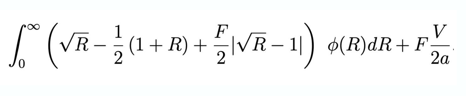
\[F^\pi=\frac{1}{E[|\sqrt{R}-1|/2]+V}\left(-2q\ E[\text{position loss}]+ \sqrt{-2qV\ E[\text{position loss}]}\right).\]
assume: liquidity providers add liquidity until they break even in expectation
Empirical Work
Lehar and Parlour (2021)
Barbon & Ranaldo (2023)
Other notables:
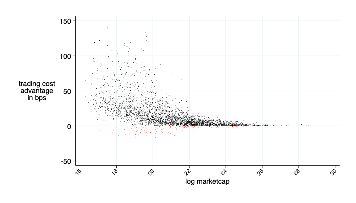
Malinova & Park (2023): AMM applied to equities would reduce trading costs by 30%
UniSwap v3
UniSwap v3 has "concentrated liquidity provision"
Just a little more institutional details
users submit liquidity positions \((u,d,p_u,p_d)\) and receive an ERC-721 (=NFT) token as a receipt
the code segments liquidity into discrete exponential intervals \([p_k,p_{k+1}]\) with \[p_k=(1+\delta)^k. ~~~(\text{numerically: }p(k)=1.0001^k)\]
it aggregates liquidity over these intervals
the pricing curve for each interval is determined by the constant product rule
intervals may be "empty"
How the price is determined
How the price is determined
\(p_d\)
\(p_u\)
\(p_0\)
we know this curve has functional form \[p^m(q)=\frac{\tilde{a}c}{(\tilde{a}-c)^2}\]
where \(\tilde{a}\) is the virtual liquidity
quick disclaimer: what follows is not how UniSwap is explained on its website etc. But the resulting maths are the same
More on UniSwap v3
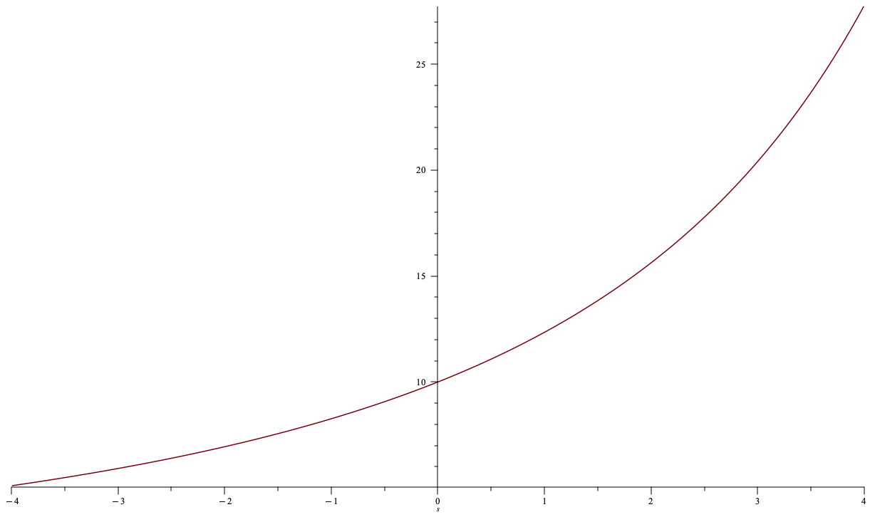
marginal "limit order book" price
\[\gamma(s)=\frac{ac}{(a-s)^2}\]
\(p_u=15\)
\(p_d=7\)
\(u=2\)
\(p_0=10\) (that's exogenous, not a choice)
Finding virtual liquidity factor \(\tilde{a}\)
marginal "limit order book" price
\[\gamma(s)=\frac{ac}{(a-s)^2}\]
\(p_u=15\)
\(p_d=7\)
\(u=2\)
\(p_0=10\) (that's exogenous, not a choice)
= find the right curve
= find the right "\(\tilde{a}\)"
Finding the fourth parameter \(\Delta c(d)\)
marginal "limit order book" price
\[\gamma(s)=\frac{ac}{(a-s)^2}\]
\(p_u=15\)
\(p_d=7\)
\(u=2\)
\(d=?\)
required cash deposit \(\Delta c(d)=\) the amount that I pay for \(d\)
Solutions
Numerical example
Want to read more?
Concerns around Automated Market Makers
a
b
c
d
e
f
g
Problem 1: Public Mempools allow sandwich (MEV) attacks
related paper: “Maximal Extractable Value and Allocative Inefficiencies in Public Blockchains”. A. Capponi, R. Jia, and Y. Wang (2023)
Problem 2: Just-In-Time Liquidity (single trade cream skimming)
X-Router
Liquidity pool
OTC
Problem 2: Just-In-Time Liquidity (at the MEV level)
X-Router
Liquidity pool
searcher/builder
balanced orders
add as much liquidity as possible
withdraw liquidity
unbalanced orders
related paper: Capponi, Jia, and Zhu (2024) "The Paradox of Just-in-Time Liquidity in Decentralized Exchanges: More Providers Can Lead to Less Liquidity"
From Vitalik Buterin's post on the topic:
https://ethresear.ch/t/improving-front-running-resistance-of-x-y-k-market-makers/1281
Theorem (Park 2023):
Hypothetical example
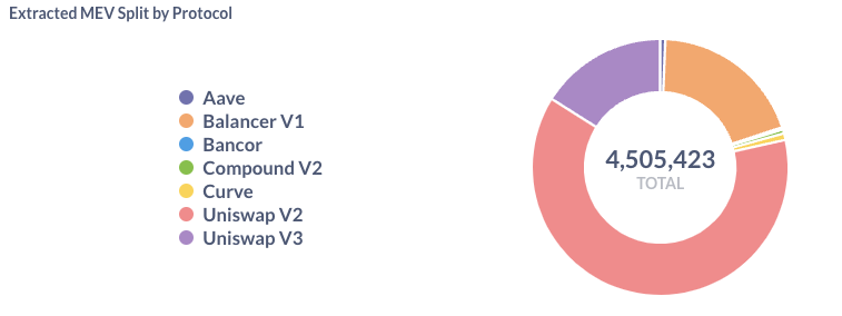
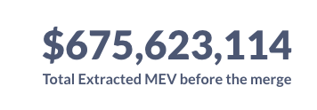
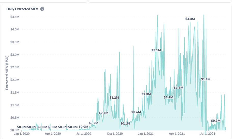
The Bigger Picture: MEV Extraction
read more at: "Battle of the Bots: Flash Loans, Miner Extractable Value and Efficient Settlement", Lehar & Parlour, 2023
The Bigger Picture and Last Words
Last Words
@financeUTM
andreas.park@rotman.utoronto.ca
slides.com/ap248
sites.google.com/site/parkandreas/
youtube.com/user/andreaspark2812/
Literature
AMM Literature: a booming field
Lehar and Parlour (2021): for many parametric configurations, investors prefer AMMs over the limit order market.
Aoyagi and Ito (2021): co-existence of a centralized exchange and an automated market maker; informed traders react non-monotonically to changes in the risky asset’s volatility
Capponi and Jia (2021): price volatility \(\to\) welfare of AMM LPs; conditions for a breakdown of liquidity supply in the automated system; more convex pricing \(\to\) lower arbitrage rents & less trading.
Capponi, Jia, and Wang (2022): decision problems of validators, traders, and MEV bots under the Flashbots protocol.
Park (2021): properties and conceptual challenges for AMM pricing functions
Milionis, Moallemi, Roughgarden, and Zhang (2022): dynamic impermanent loss analysis for under constant product pricing.
Hasbrouck, Rivera, and Saleh (2022): higher fee \(\Rightarrow\) higher volume
Empirics:
Lehar and Parlour (2021): price discovery better on AMMs
Barbon and Ranaldo (2022): compare the liquidity CEX and DEX; argue that DEX prices are less efficient.
payments network
Stock Exchange
Clearing House
custodian
custodian
beneficial ownership record
seller
buyer
Broker
Broker
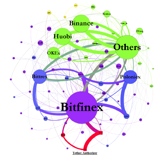
IS BITCOIN REALLY UN-TETHERED? JOHN M. GRIFFIN and AMIN SHAMS
Journal of Finance 2020
Figure 1. Aggregate Flow of Tether between Major Addresses
marginal pricing function
quantity \(q\)
price \(p^m(q)\)
Illustration of pricing
Some Pricing Rules from Traditional Markets: Limit Order Book
\[\Delta c(q)=\int_0^q\rho(s) ds.\]
Returns to Liquidity Provision
For fixed balanced volume \(V\) and fee \(F\)
Competitive liquidity provision
Basics of Liquidity Provision
\[\text{LP payoff}=\text{what I sold it for}-\text{value of net position}+\text{fee income}\]
see Lehar and Parlour (2023), Barbon & Ranaldo (2022).
(incremental) adverse selection loss when the return is \(R\)
fees earned
on informed
fees earned
on balanced flow
for reference:
positional loss
Basics of Liquidity Provision
\[\frac{1}{\text{initial deposit}}\int_0^\infty(\Delta c(q^*)-q^*p_t(R)+F \cdot \Delta c(q^*))~\phi(R)dR +\frac{F p_0 V}{\text{initial deposit}}\ge 0\]
\[\int_0^\infty\left(\frac{\Delta c(q^*)-q^*p_t(R)}{\text{initial deposit}} +F \cdot \frac{\Delta c(q^*)}{\text{initial deposit}}\right)~\phi(R)dR +\frac{F p_0 V}{\text{initial deposit}}\ge 0\]
closed form functions of \(R\) only
(see Barbon & Ranaldo (2022))
\[\underbrace{F \int DV \mu(DV) }_{\text{fees earned on}\atop \text{balanced flow}}+\int_0^\infty\underbrace{(\Delta c(q^*)-q^*p_t(R)}_{\text{adverse selection loss} \atop \text{when the return is {\it R}}} +\underbrace{F \cdot \Delta c(q^*))}_{\text{fees earned}\atop \text{from arbitrageurs}}~\phi(R)dR \ge 0.\]
Basics of Liquidity Provision
\(\Rightarrow\) \(\Delta c(q^*)-q^*p_t(R)\) is also referred to as the "impermanent loss" or "divergence loss"
\(\Delta c(q^*)-q^*p_t(R)=\underbrace{p_t(R)\times(a-q^*) +c+\Delta c(q^*)}_{\text{value of liquidity deposit}}-\underbrace{(p_t(R)a+c)}_{\text{value of buy-} \atop \text{and-hold position}}\)
see Milionis, Moallemi, Roughgarden, and Zhang (2022) for a dynamic analysis of impermanent loss
Basics of Liquidity Provision
Liquidity provision measured as "collective" deposit \(\alpha\) of token's market cap as function of
\[E[\text{DL}(R)]+F\cdot E[\text{another function of }R]+F\cdot \frac{\text{E[dollar volume]}}{\text{initial deposit}}\ge 0.\]
\[\text{what I sold it for}-\text{value of net position}+\text{fee income} \ge 0 \]
The Decision of the Liquidity Demander
\[F^\pi=\frac{1}{E[|\sqrt{R}-1|/2]+E[DV]}\left(-2q\ E[\text{DL}]+ \sqrt{-2qE[DV]\ E[\text{DL}]}\right).\]
this is from Malinova and Park (2023); similar result is in Hasbrouk, Riviera, Saleh (2023)
Model Summary
The Pricing Function
Liquidity Deposit \(\Rightarrow\) slope of the price curve
The Pricing Function (just a little more)
The Pricing Function (almost done, just one more thing)
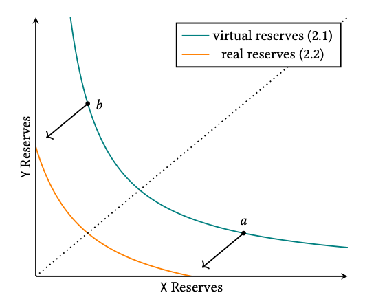
AMMs continue to evolve: UniSwap v3
Basic idea:
Source:" Uniswap v3 Core," Adams, Zinsmeister, Salem, Keefer, Robinson (2021)
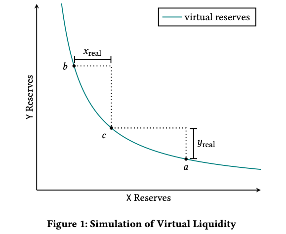
Some UniSwap v3 maths (Barbon & Ranaldo 2023)
Source: Elsts (2021) "Liquidity Math in UniSwap v3"
\(X\)
\(Y\)
normal trade: sell \(x\) \(\to\) get \(y'\)
\(Y-y'\)
\(X+x\)
front-running:
\(Y-y'-y''\)
\(X+2x\)
\(y'>y''~\Rightarrow\)
front-running is intrinsically profitable
Disclaimer:
Problems:
lesser problem because
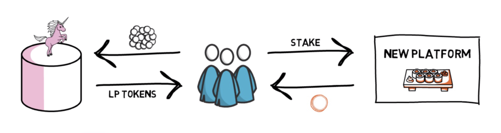
Common solution: create a reward token! Here's how this works
Step 4: users receive a reward token based on the time that they lock up the "receipt" token
Step 3: users lock up the "receipt" token in a smart contract
Step 2: users contribute liquidity and get a "receipt" token
Step 1: create reward tokens and deposit into a smart contract
borrow
provide collateral
Application: Pool-based borrowing and lending
Same problems as with trading:
But: in contrast to trading, here you need both!
liquidity \(\nearrow\)
volume \(\nearrow\)
protocol fees \(\nearrow\)
token value \(\nearrow\)
Platform economics is tricky:
Without intermediaries:
platform economics!
incentives for both?
What value do these tokens have?
Vampire Attacks and Other Shenanigans
Source: https://finematics.com/vampire-attack-sushiswap-explained/
another common trick:
By Andreas Park
Presentation for CBER-DFI Crypto-Economics Summer School 2024


