


Andreas Park PRO
Professor of Finance at UofT
Katya Malinova and Andreas Park
Agenda
Some Motivation
Basic Idea
payments network
Stock Exchange
Clearing House
custodian
custodian
beneficial ownership record
seller
buyer
Broker
Broker
Broker
Exchange
Internalizer
Wholeseller
Darkpool
Venue
Settlement
New institutions!
Key Components
Overview
Roadmap for the rest of the talk
Automated Market Makers
Basics of Liquidity Provision
in traditional markets: bid-ask spread
The Decision of the Liquidity Provider
AMM Pricing
Constant Liquidity (Product) AMM
The Decision of the Liquidity Provider
Deposit \(\Rightarrow\) slope of the price curve
AMM Properties
AMM Properties
Constant liquidity pricing function is not "regret free" - LPs always lose (Park 2023)
Liquidity Provider gains/losses
for orientation:
Another way to look at the net loss:
Liquidity Provision
Theory Overview
Big Picture for Liquidity Provision
\[\text{what you earn from dumb people}-\text{what you lose against smart people}\ge0\]
Big Picture for Liquidity Provision
\[\underbrace{F\times v}_{\text{earn on dumb people}} +\underbrace{F\times \Delta (q^*)+\Delta c(q)-p_tq}_{\text{loss from smart people}}\ge 0\]
Liquidity Provision in AMMs
Big Picture for Liquidity Provision
Liquidity Provider Expected Return
Expressing terms:
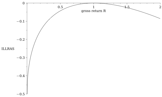
\[\int\limits_0^\infty\left(\sqrt{R}-\frac{1}{2}\left(1+R\right)+\frac{F}{2}|\sqrt{R}-1|\right)~\phi(R)dR+F\frac{V}{2a}.=0\]
Equilibrium Liquidity Supply
Gives us an equilibrium deposit \(a^*\)
\[a^*=\frac{F V}{2}\underbrace{\left(-F\times E[|\sqrt{R}-1|/2]-E[\text{ILLRAS}]\right)^{-1}}_{=:C^\mathsf{CP}(\phi,F)^{-1}}.\]
liquidity provider choice variable: the initial deposit
The Decision of the Liquidity Provider
We express \(a\) as the fraction of shares outstanding:
\[a=\alpha S, ~~~\alpha\in[0,1].\]
The equilibrium value is (also) the largest deposit so that liquidity providers want to participate. Hence
\[\overline{\alpha}=\min\left\{1,\frac{F V}{2S}\frac{1}{C^\mathsf{CP}(\phi,F)}\right\}\]
The Decision of the Liquidity Demander
The Optimal Fee for Liquidity Providers is not Zero
Model Summary
How we think of the Implementation of an AMM for our Empirical Analysis
Approach: daily AMM deposits
Assumptions for Empirical Investigation
Presentation of the Results in THREE steps
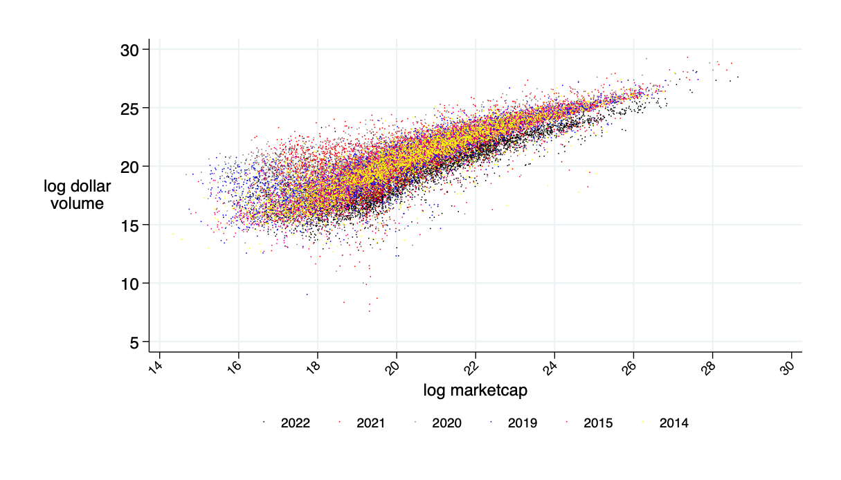
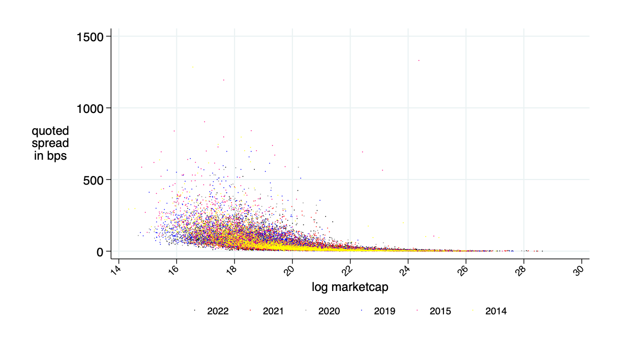
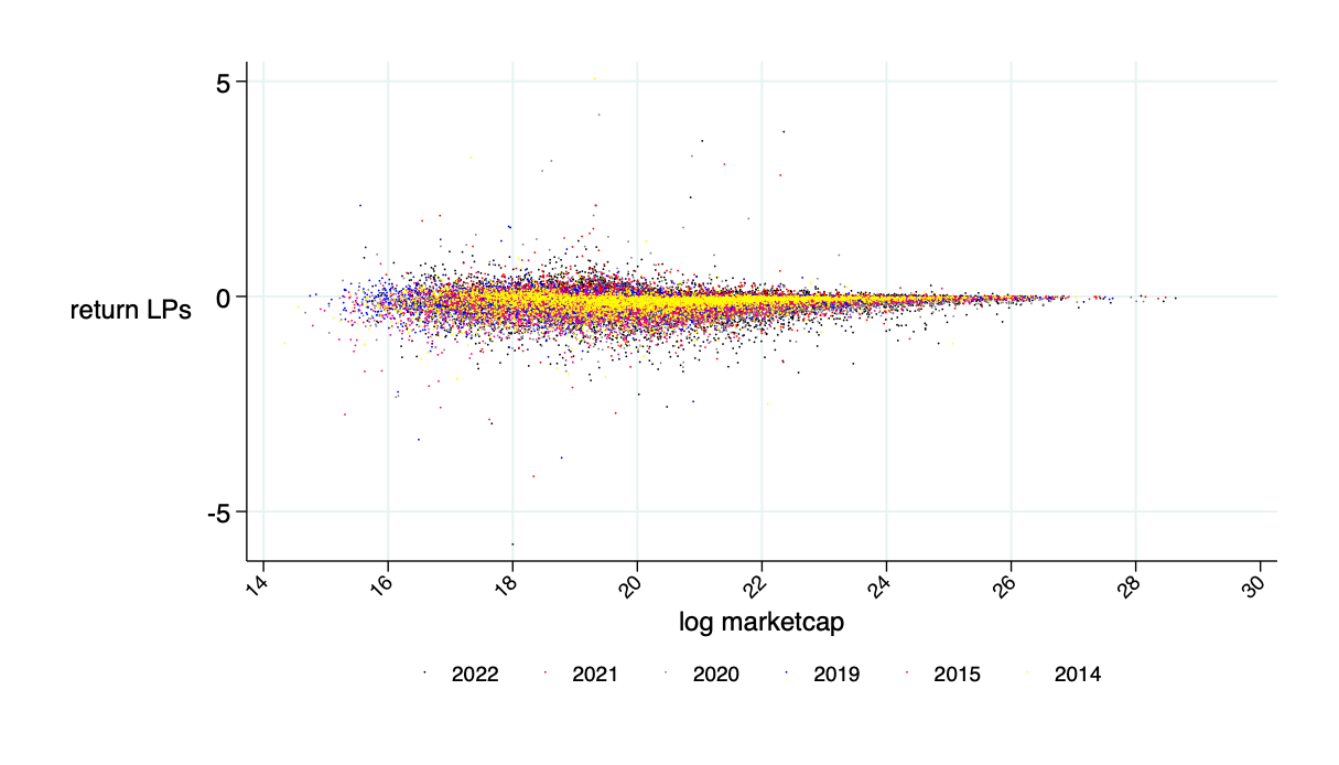
Data-Peeking
Getting a Sense of the Relationships
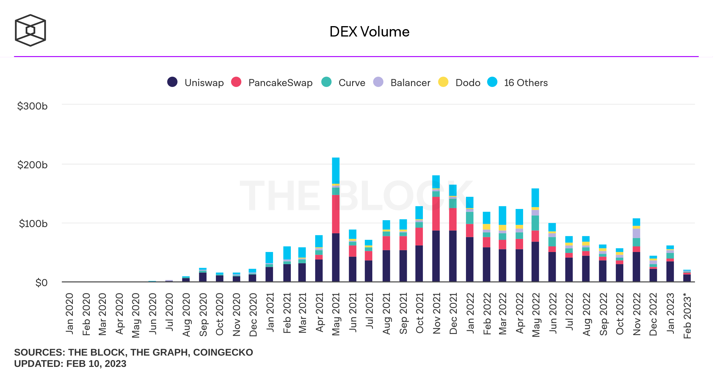
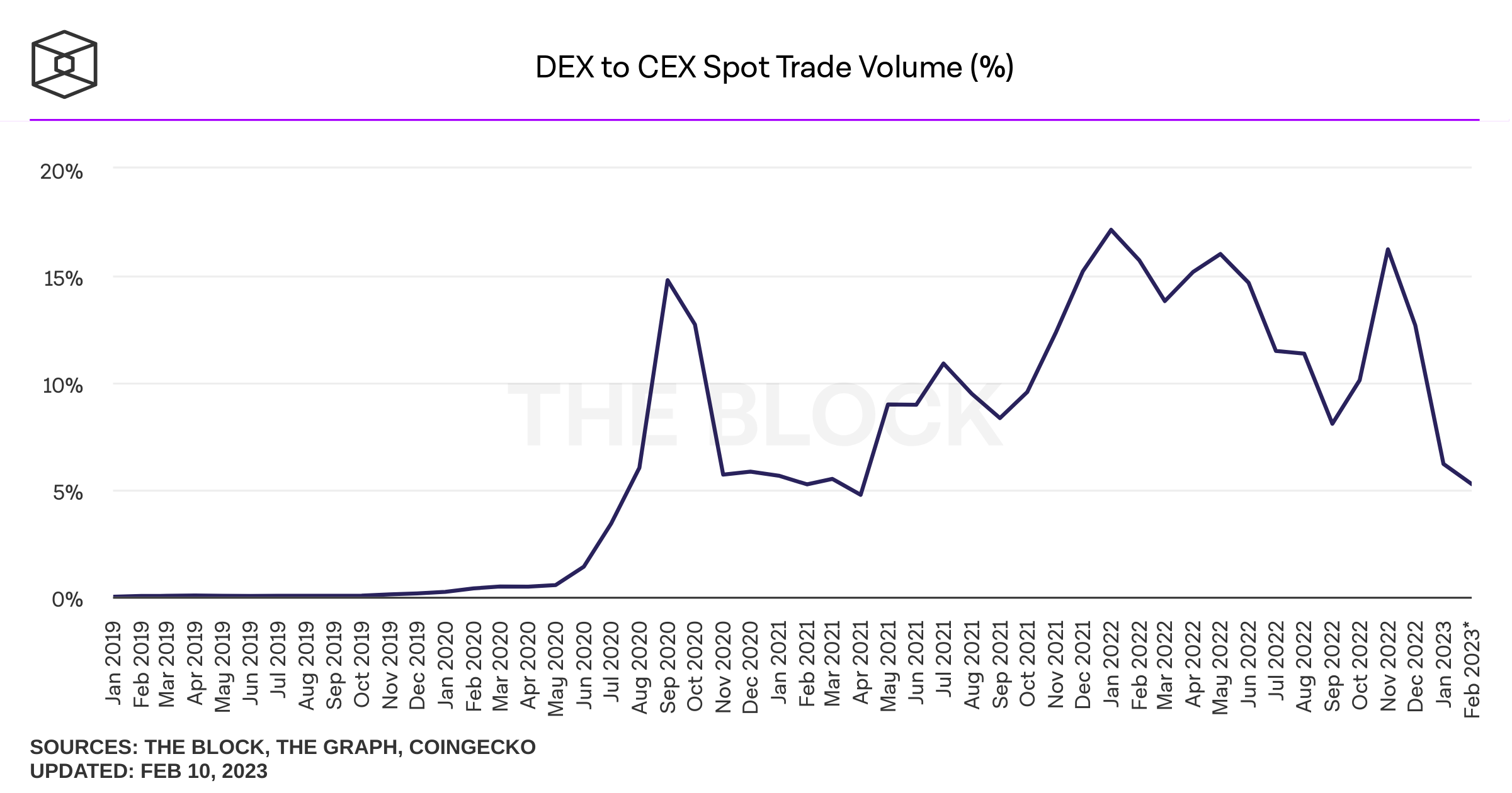
some volume may be intermediated
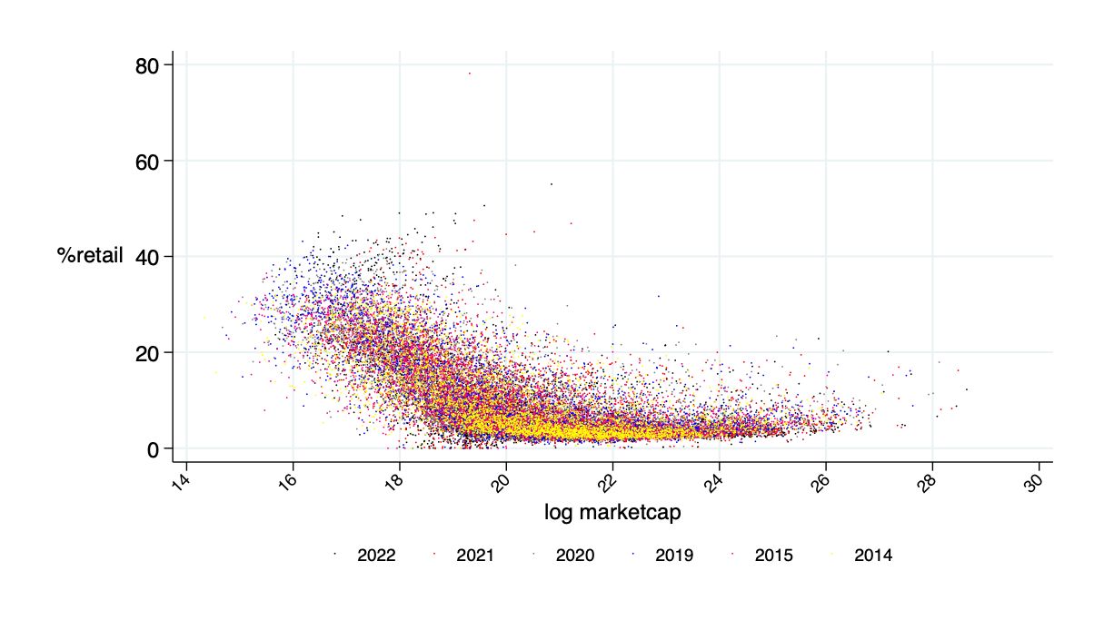
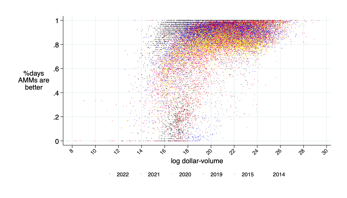
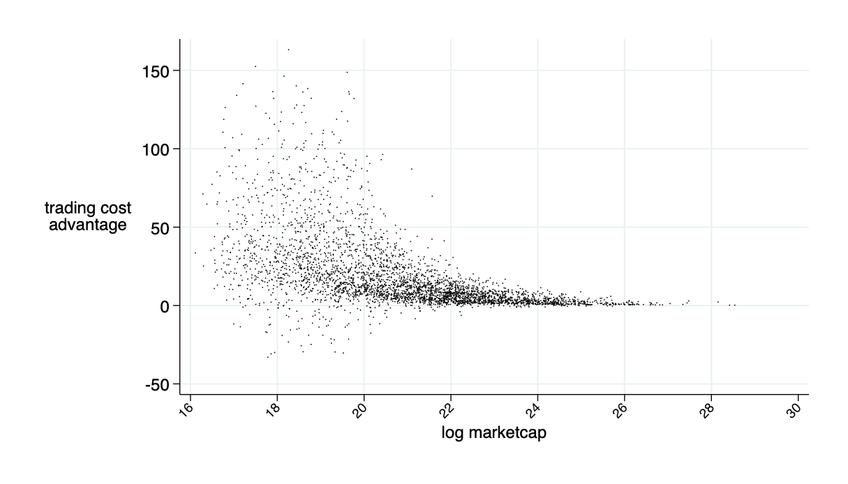
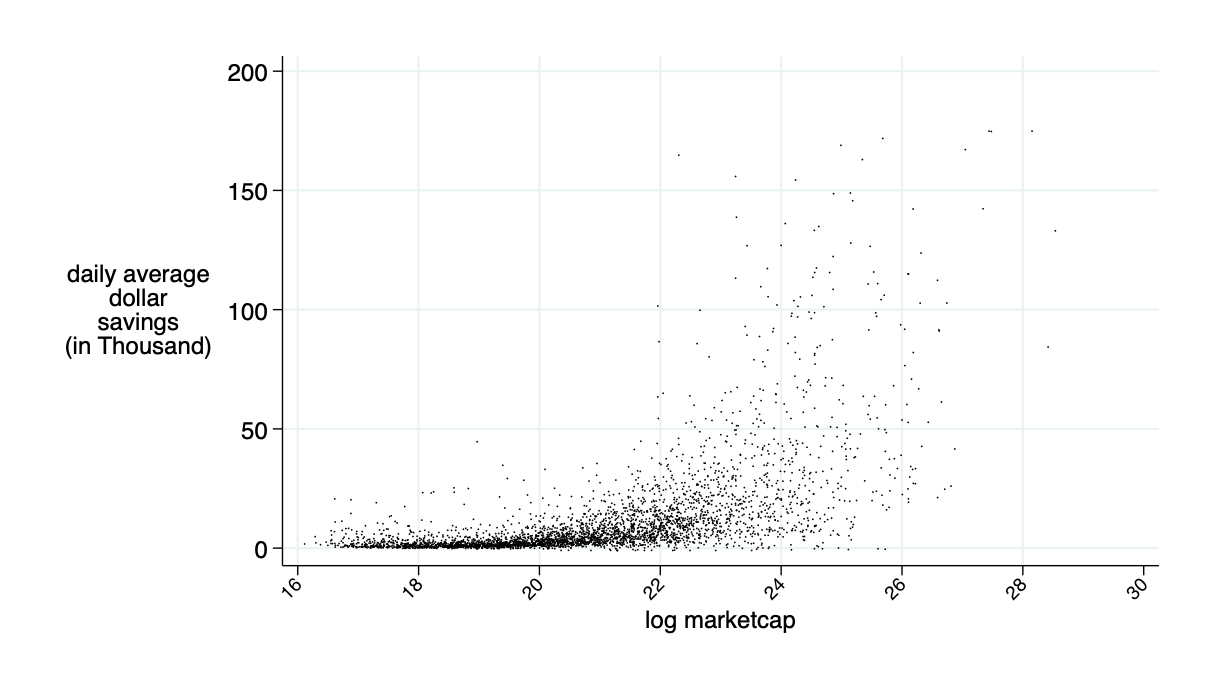
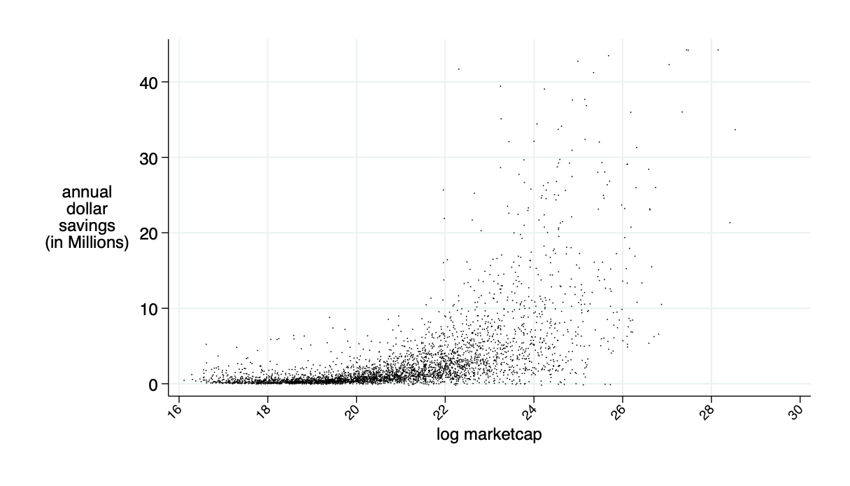
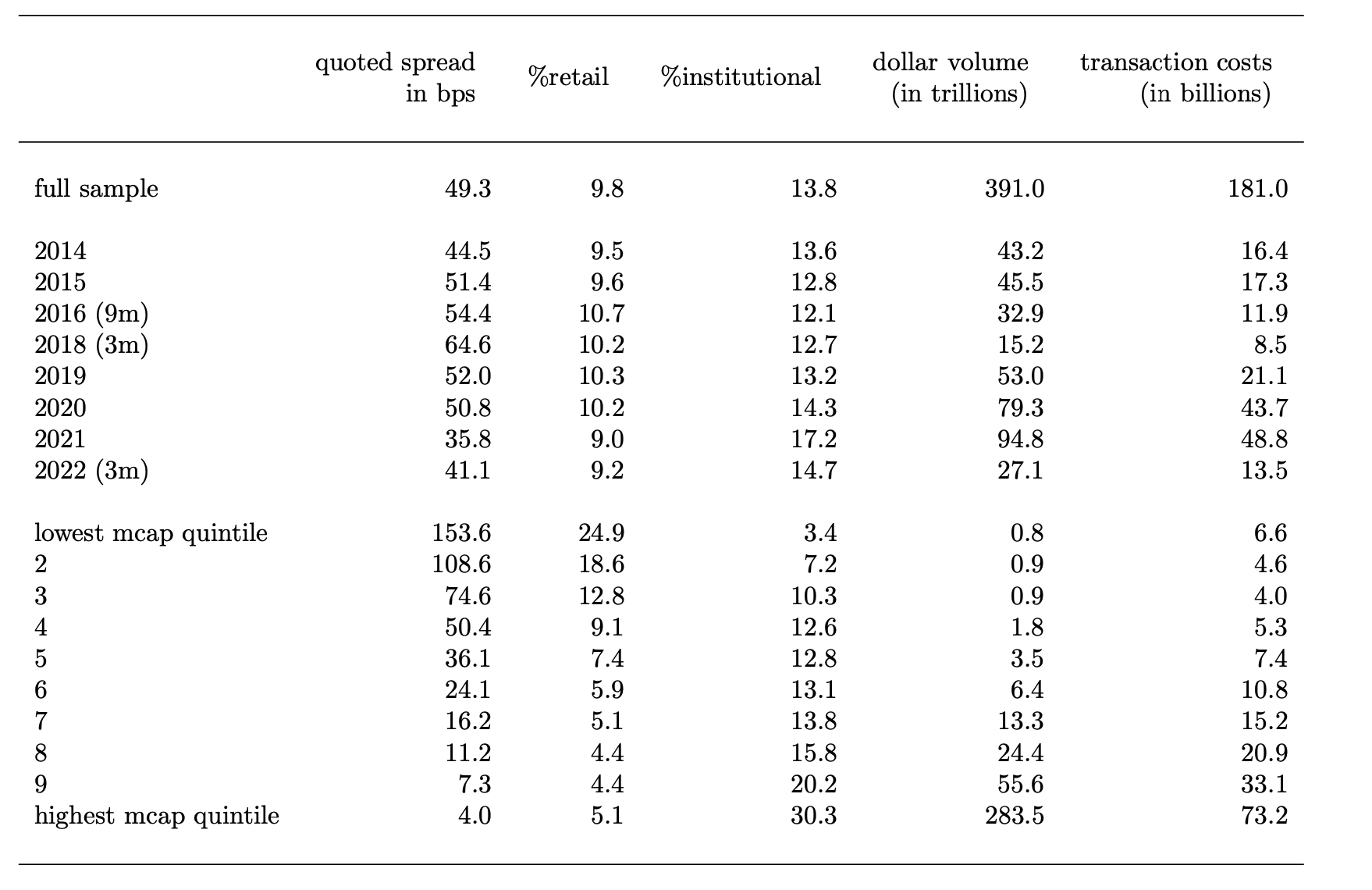
Some Cross-Sectional Relationships
retail = as defined in "Tracking Retail Investor Activity" Boehmer, Jones, Zhang, and Zhang (JF 2021)
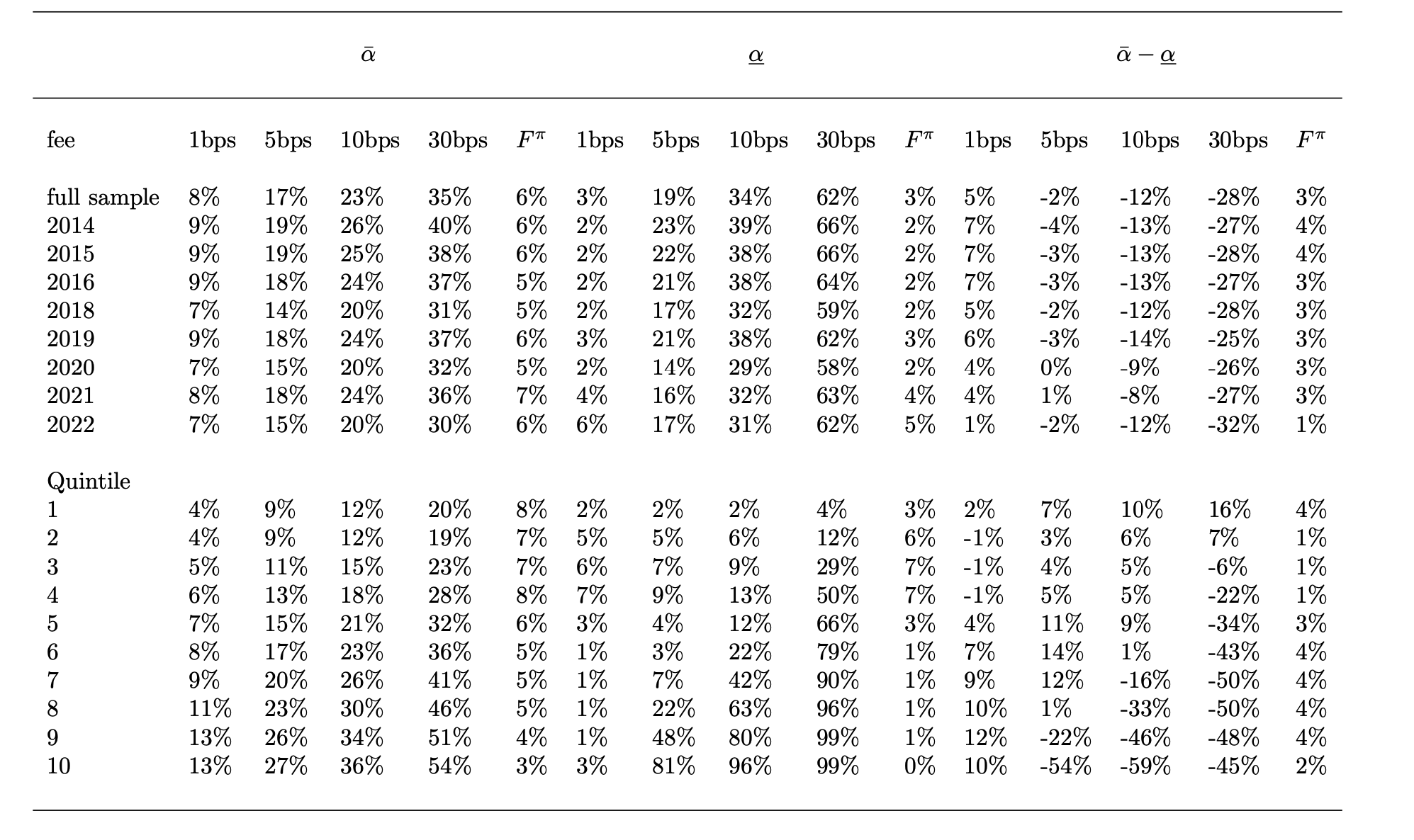
Threshold for Feasibility: \(\overline{\alpha}-\underline{\alpha}\)
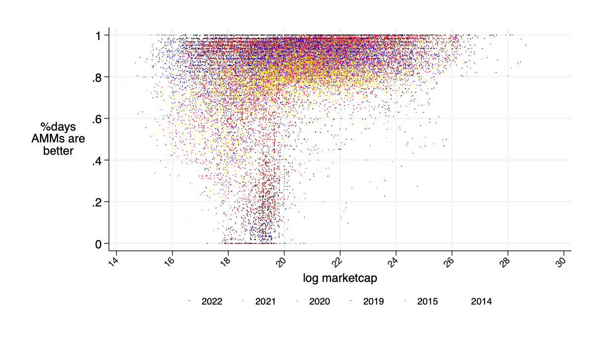
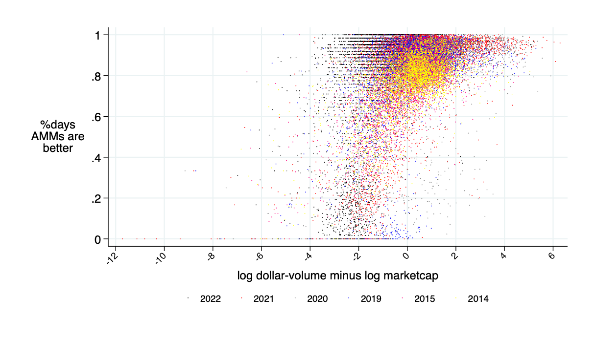
Days with feasibility
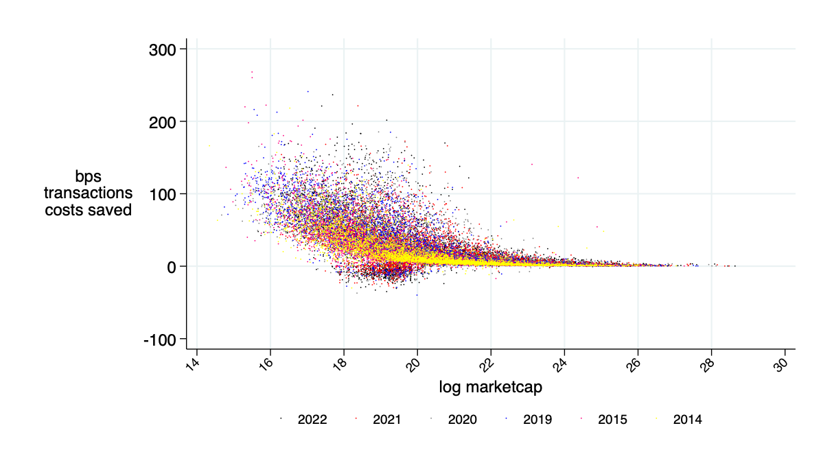
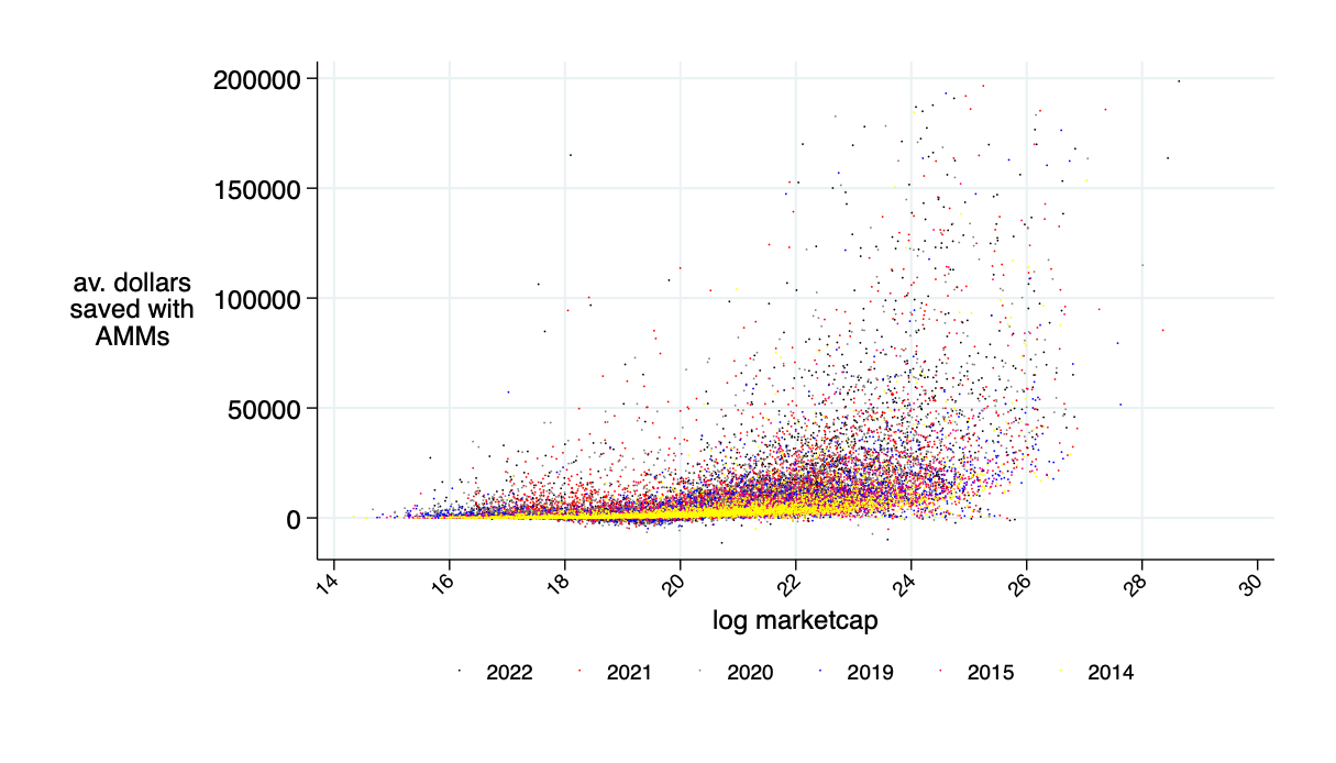
Average Benefit of AMM per day
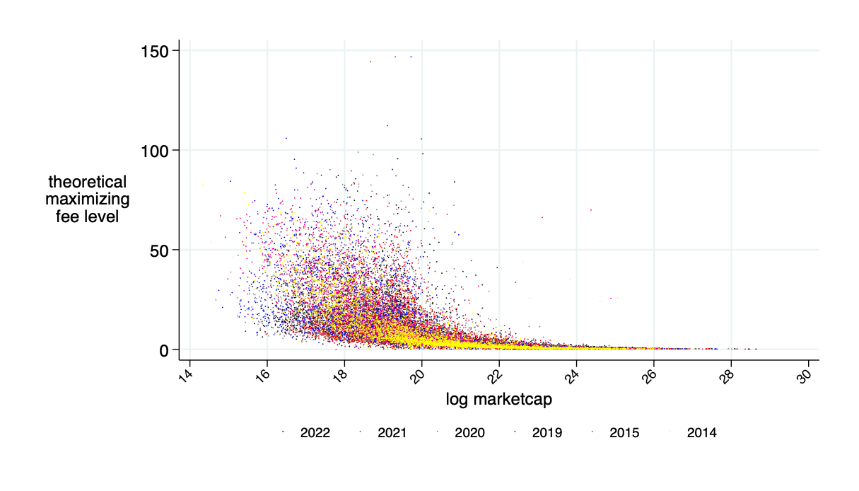
Optimally Designed AMMs
Assumptions for Optimality
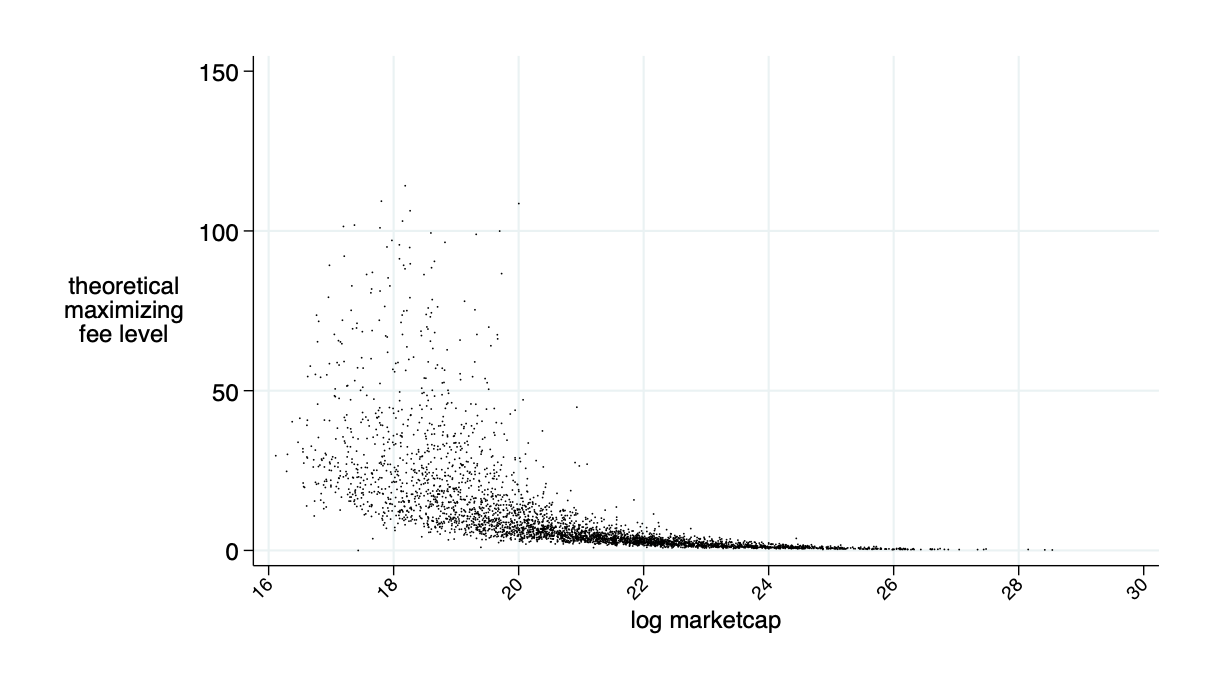
The optimal fee \(F^\pi\) maximizes
\[\pi(F)=\sigma-\frac{q}{\bar{\alpha}S-q}-F\]
with solution (no expectations)
\[F^\pi=\frac{-2qp\ \text{ILLRAS}}{V}+ \sqrt{\frac{-2qp\ \text{ILLRAS}}{V}}\]
Optimal fee \(F^\pi\)
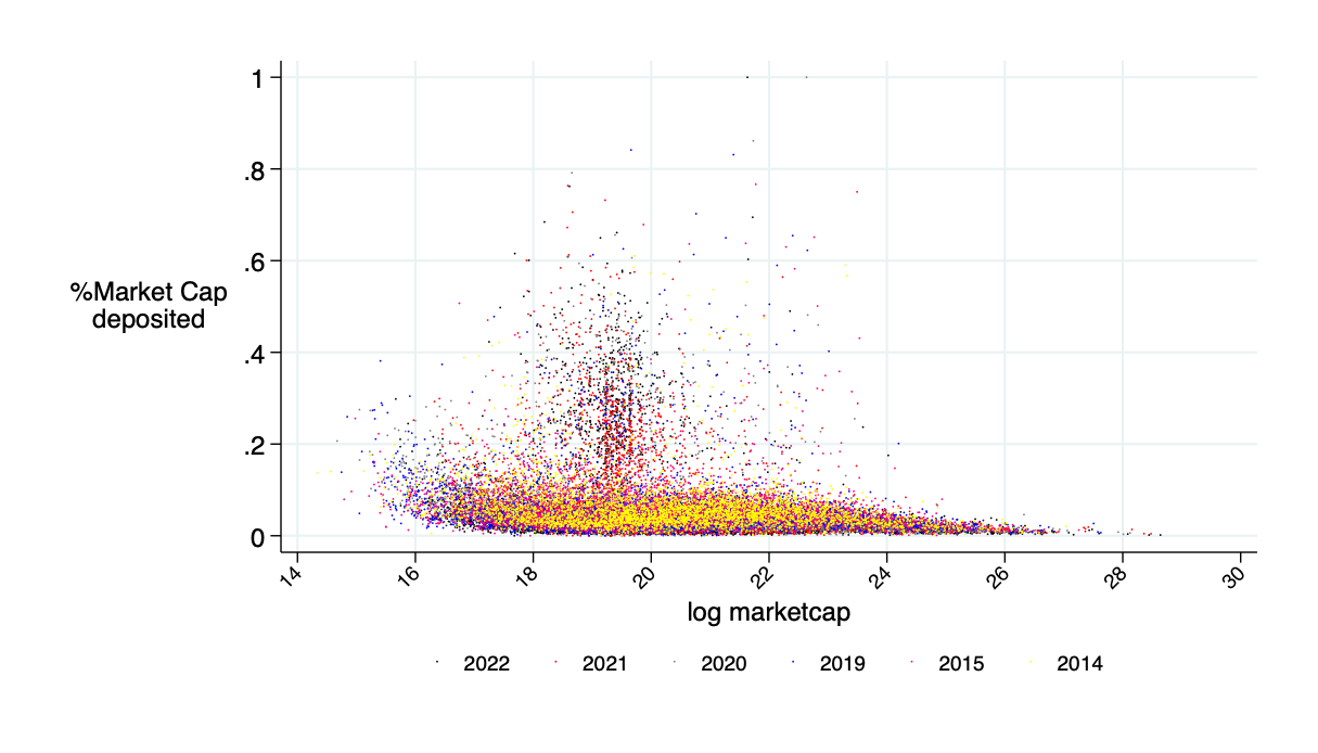
\(\overline{\alpha}\) for \(F=F^\pi\)
\(\approx\) 200 low-volume stocks (avg volume 20% of rest)
quoted spread minus AMM price impact minus AMM fee (all measured in bps)
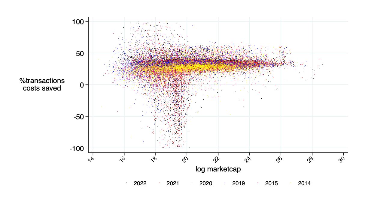
relative savings:
fees paid in AMM/fees paid with spreads
average benefits liquidity provider in bps (average=0)
AMMs with expectations
Assumptions for Optimality
Two approaches
Implementation notes:
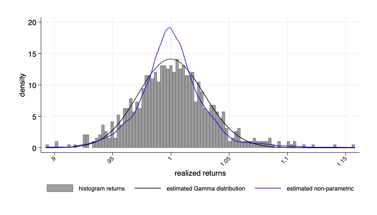
Return distribution example: Microsoft
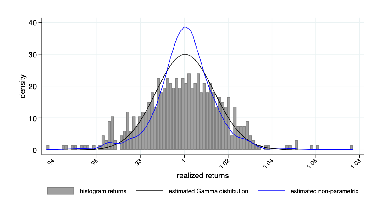
Return distribution example: Tesla
average savings: 18 bps
average daily: $12K
average annual: $2.95 million
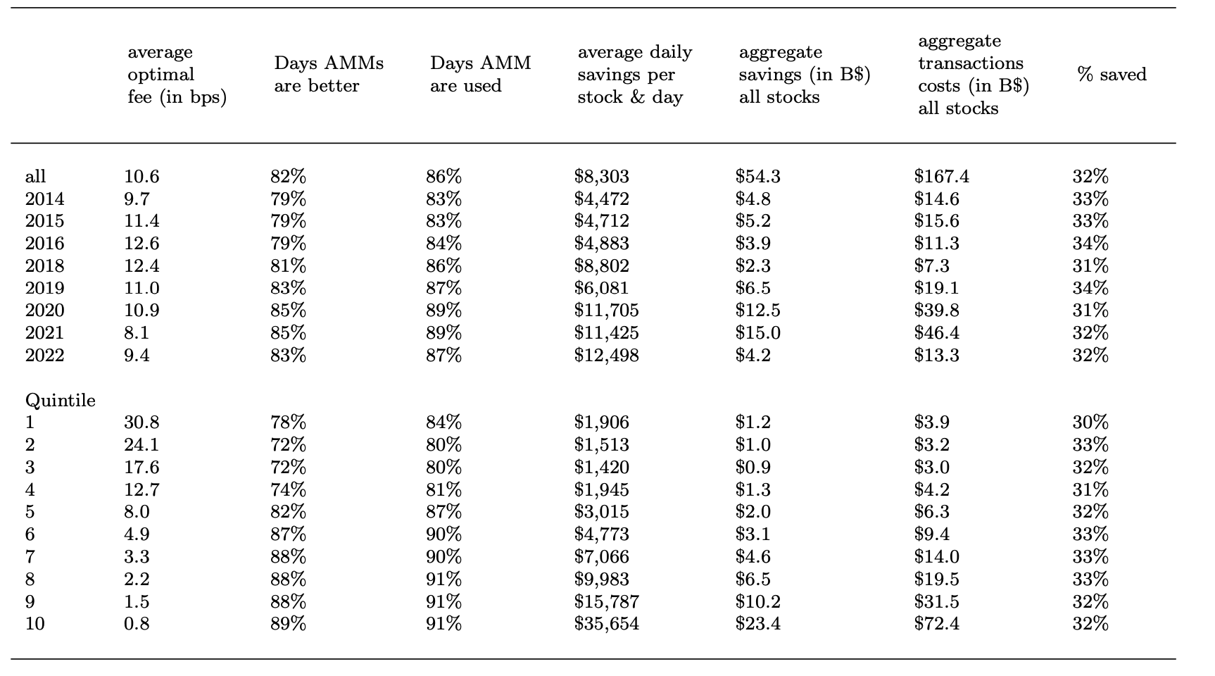
Some Numbers
(based on "yesterday's")
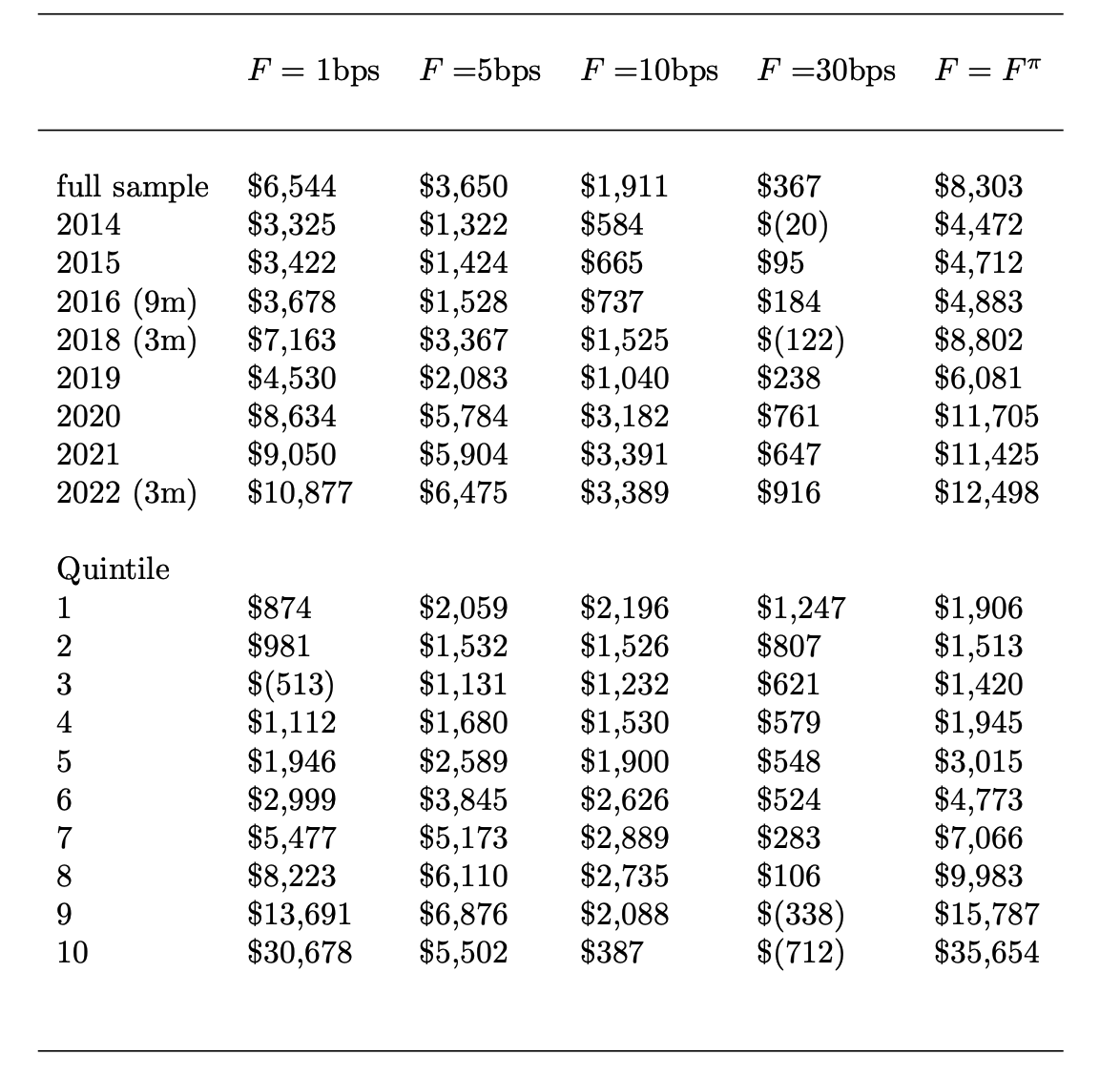
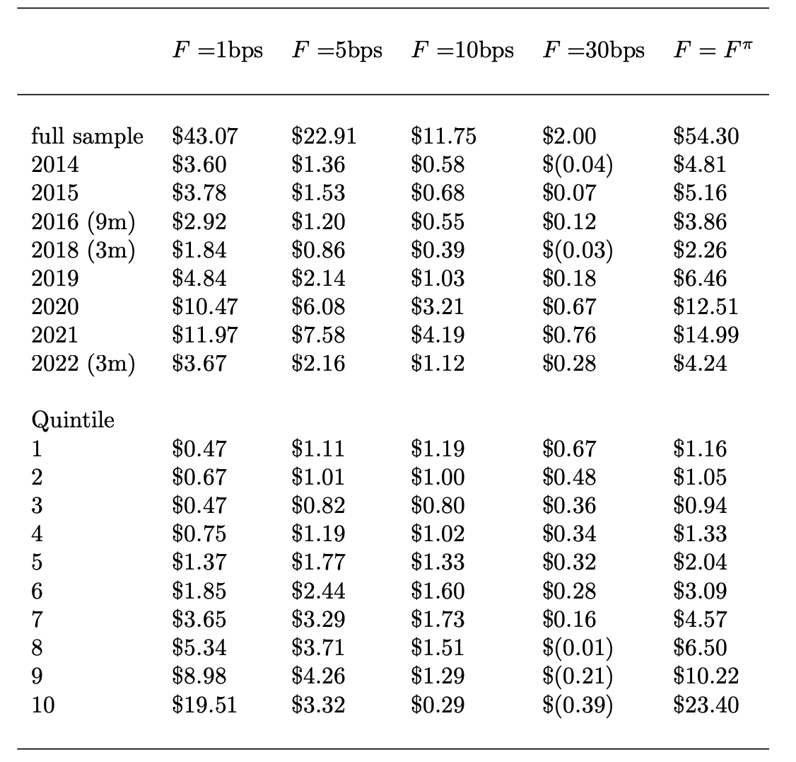
average per stock and day benefit for liquidity takers
aggregate benefit for liquidity takers (in B$)
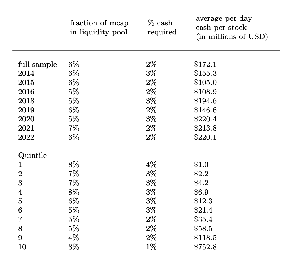
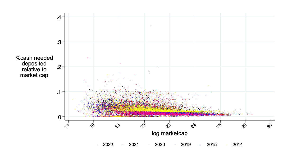
Sidebar: Capital Requirement
Deposit Requirements
Literature
AMM Literature: a booming field
Lehar and Parlour (2021): for many parametric configurations, investors prefer AMMs over the limit order market.
Aoyagi and Ito (2021): co-existence of a centralized exchange and an automated market maker; informed traders react non-monotonically to changes in the risky asset’s volatility
Capponi and Jia (2021): price volatility \(\to\) welfare of AMM LPs; conditions for a breakdown of liquidity supply in the automated system; more convex pricing \(\to\) lower arbitrage rents & less trading.
Capponi, Jia, and Wang (2022): decision problems of validators, traders, and MEV bots under the Flashbots protocol.
Park (2021): properties and conceptual challenges for AMM pricing functions
Milionis, Moallemi, Roughgarden, and Zhang (2022): dynamic impermanent loss analysis for under constant product pricing.
Hasbrouck, Rivera, and Saleh (2022): higher fee \(\Rightarrow\) higher volume
Empirics:
Lehar and Parlour (2021): price discovery better on AMMs
Barbon and Ranaldo (2022): compare the liquidity CEX and DEX; argue that DEX prices are less efficient.
The Bigger Picture. Obstacles, Solutions, and Last Words
Where do the savings come from?
Obstacles
Summary
@financeUTM
andreas.park@rotman.utoronto.ca
slides.com/ap248
sites.google.com/site/parkandreas/
youtube.com/user/andreaspark2812/
By Andreas Park


