Introduction to galaxy clustering
Arnaud de Mattia
CEA Saclay, Irfu/DPhP
Goals
- broad overview of the domain
- keys to easily read and criticize clustering analysis papers
- to get a bit deeper: Percival 2013, Percival 2018
- Past and current surveys
- Clustering observables
- Spectroscopic surveys and systematics
- Large-scale structure formation
- BAO and RSD theory models
- Current constraints
- Other clustering analyses
Goals
- broad overview of the domain
- keys to easily read and criticize clustering analysis papers
- to get a bit deeper: Percival 2013, Percival 2018
Goals
- broad overview of the domain
- keys to easily read and criticize clustering analysis papers
- to get a bit deeper: Percival 2013, Percival 2018
- Past and current surveys
- Clustering observables
- Spectroscopic surveys and systematics
- Large-scale structure formation
- BAO and RSD theory models
- Current constraints
- Other clustering analyses
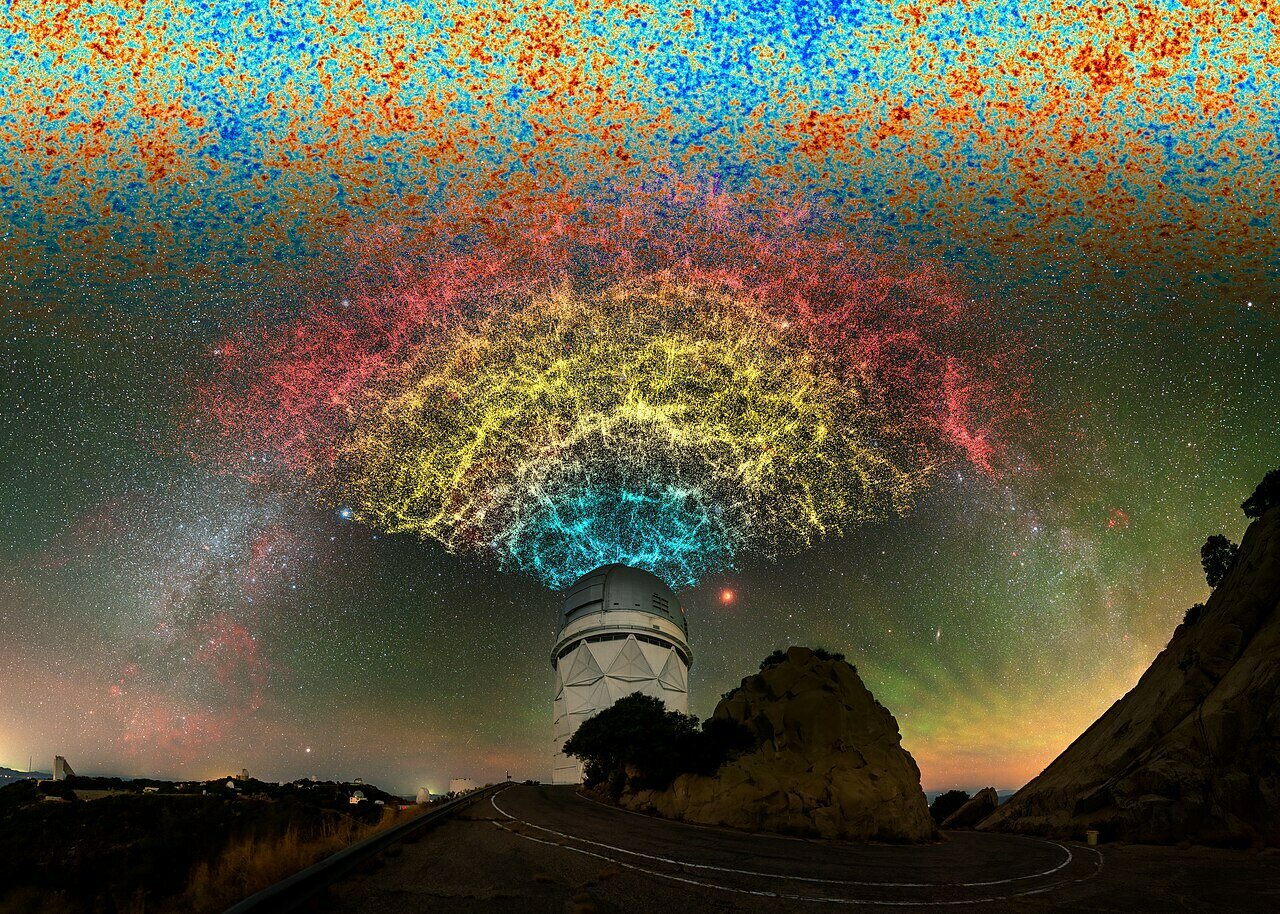
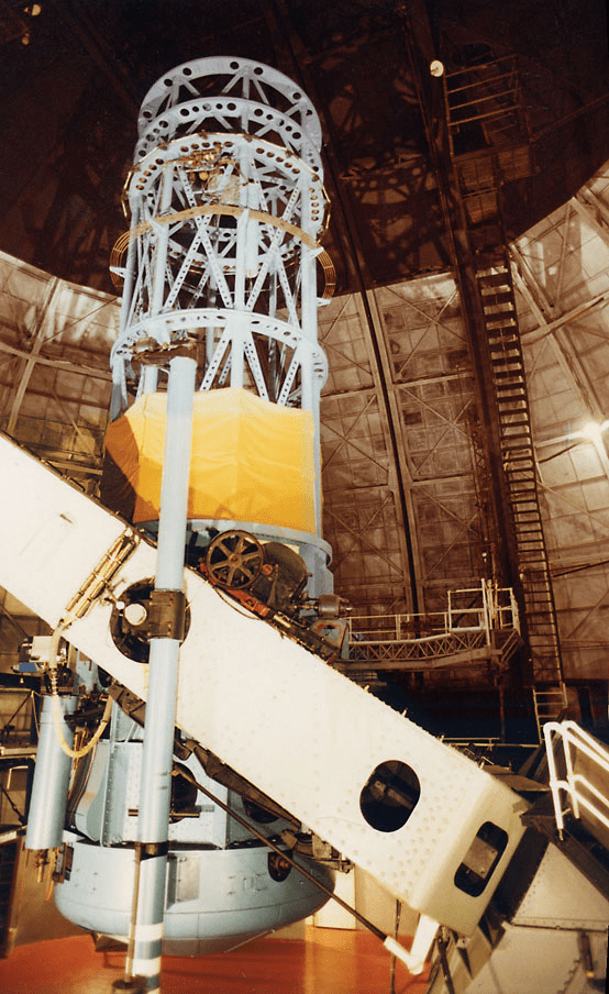
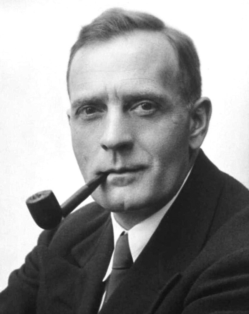
- 1924, Mount Wilson: Edwin Hubble shows the existence of
galaxies (previoulsy nebulae) using cepheids
Cataloguing galaxies
Cataloguing galaxies
- 1924, Mount Wilson: Edwin Hubble shows the existence of
galaxies (previously nebulae) using cepheids - early imaging surveys carried out with photometric plates:
- 1949 - 1958: Palomar Observatory Sky Survey (POSS I)
- 1974 - 1999: UKST sky surveys, Siding Spring, Australia
- 1985 - 2000: POSS II
Cataloguing galaxies
-
galaxy catalogs:
- 1961 - 1968: Zwicky Catalog of galaxies based on POSS I
- 1967: Lick catalog of 1M galaxies
-
numerization:
- 1994: Digitized Sky Survey, scanning of POSS I/II and UKST: 102 CD-roms
- 1997 - 2001: 2MASS (Arizona, USA, and Chile) 3-band photometric survey
- 1924, Mount Wilson: Edwin Hubble shows the existence of
galaxies (previously nebulae) using cepheids - early imaging surveys carried out with photometric plates:
- 1949 - 1958: Palomar Observatory Sky Survey (POSS I)
- 1974 - 1999: UKST sky surveys, Siding Spring, Australia
- 1985 - 2000: POSS II
How to go 3D?
R.A.
Dec.
R.A.
Dec.
z
With spectroscopic surveys!
More specifically:
- broad-band photometric surveys: \(\sigma(z) \sim 0.03 (1 + z)\)
- spectroscopic surveys: \(\sigma(z) \sim 0.0001 (1 + z)\)
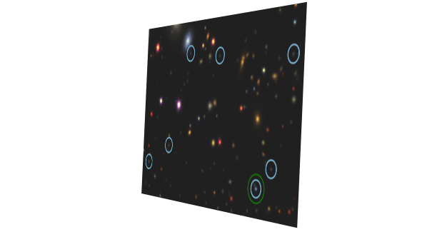
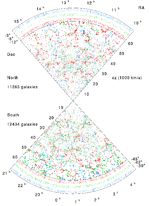
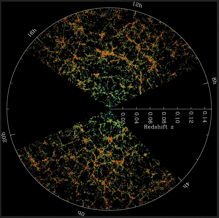
CfA redshift surveys
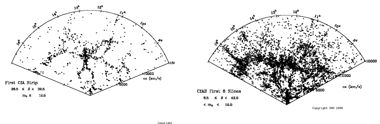
Mesurement of galaxy redshifts using a spectrograph.
- redshifts of galaxies from updated Zwicky catalogs
- 1977 - 1982: CfA I, 1100 redshifts, structures formed by galaxies
- 1985 - 1995: CfA II, 18k redshifts, Great Wall (Geller and Huchra 1989) at \(z \simeq 0.03\)
CfA redshift surveys
Mesurement of galaxy redshifts using a spectrograph.
- redshifts of galaxies from updated Zwicky catalogs
- 1977 - 1982: CfA I, 1100 redshifts, structures formed by galaxies
- 1985 - 1995: CfA II, 18k redshifts, Great Wall (Geller and Huchra 1989) at \(z \simeq 0.03\)
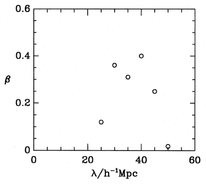
First cosmological constraints
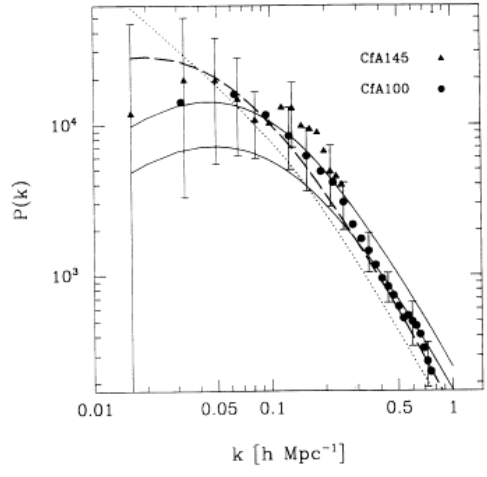
- Vogeley et al. 1992 with CfA: inconsistency with CDM model at 99% (propose oCDM)
- Cole et al. 1994 with IRAS (infrared space telescope) data (15k redshifts): first measurement of anisotropy (\(\beta\) parameter) w.r.t. line-of-sight (due to redshift-space distortions)
First cosmological constraints
- Vogeley et al. 1992 with CfA: inconsistency with CDM model at 99% (propose oCDM)
- Cole et al. 1994 with IRAS (infrared space telescope) data (15k redshifts): first measurement of anisotropy (\(\beta\) parameter) w.r.t. line-of-sight (due to redshift-space distortions)
Since the 90's, multi-object spectroscopy
- How to speed up redshift surveys? Many spectra at once!
- Demonstrators in the 80's (MEDUSA, FOCAP)
- Las Campanas Redshift Survey (1991 - 1996)
- 2.5 m Dupont Telescope at LCO, Chile, 50 fibers
- 26k galaxies at \(z < 0.2\) over \(700\;\mathrm{deg}^2\)
CfA
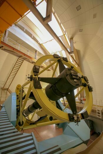
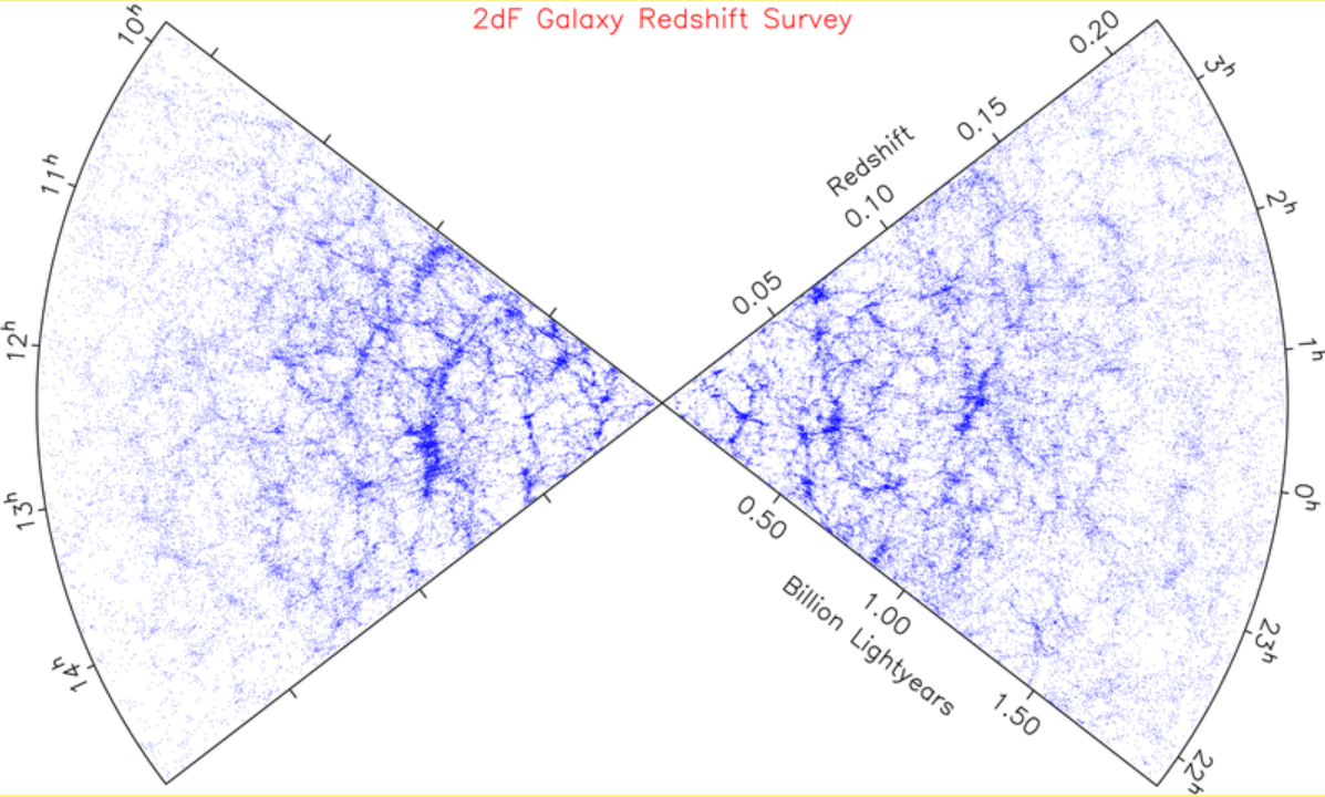
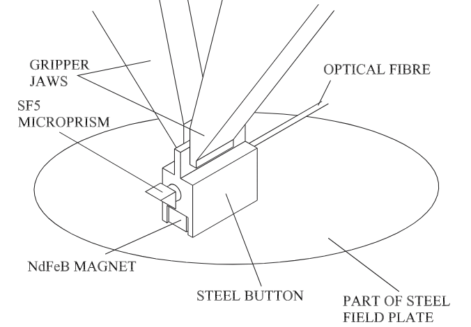
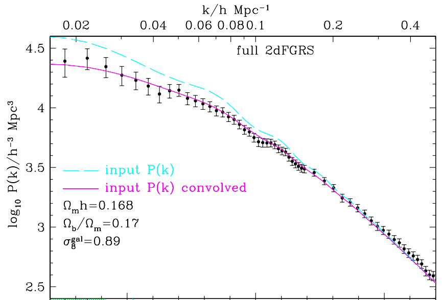
2dFGRS
- 2dF Galaxy Redshift Survey (1997 - 2002)
- Anglo-Australian 3.9-m telescope (AAT), 400 fibers
- 221k galaxies at \(z < 0.3\) over \(1800\;\mathrm{deg}^2\)
2dFGRS
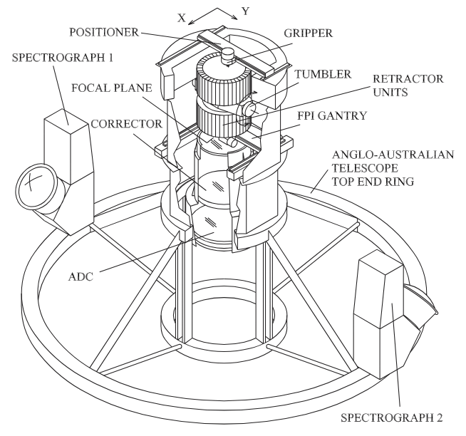
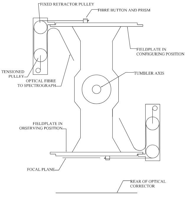
single robotic positioner
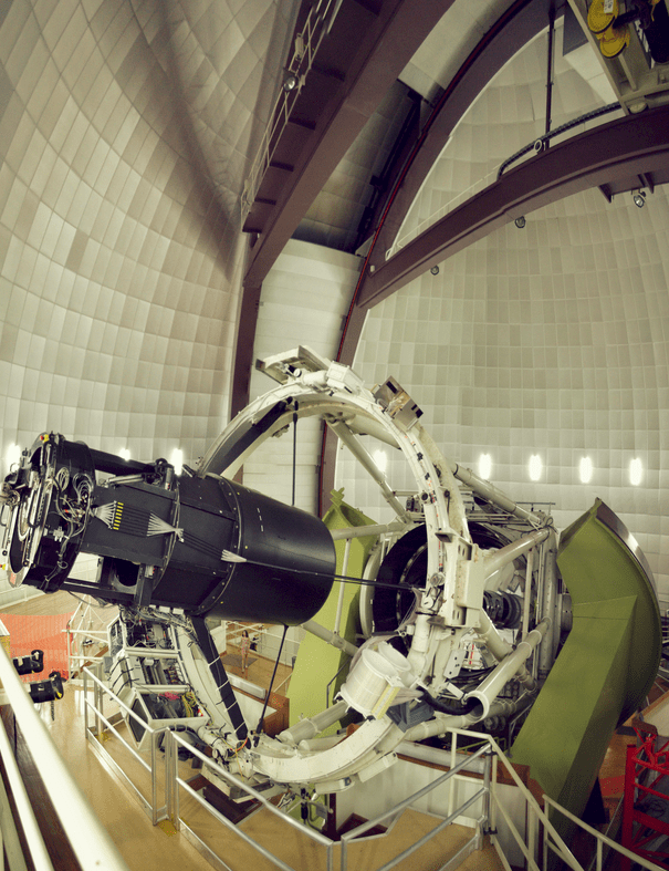
SDSS I-II
-
SDSS-I and II (2000 - 2008)
- 2.5-m telescope at Apache Point Observatory, 500 fibers
- Main Galaxy Sample (MGS), 800k galaxies at \(z < 0.25\) over \(8000\;\mathrm{deg}^2\)
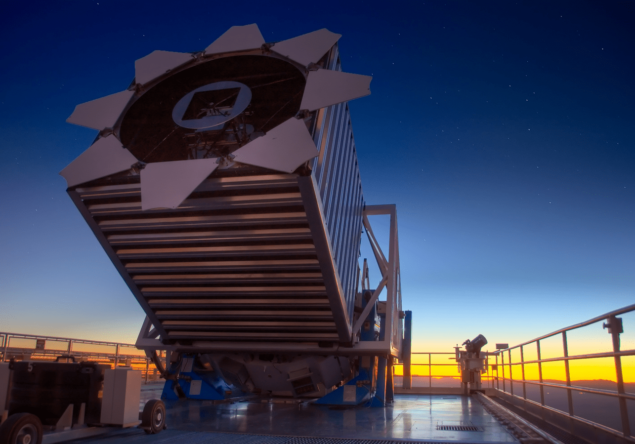
SDSS I-II
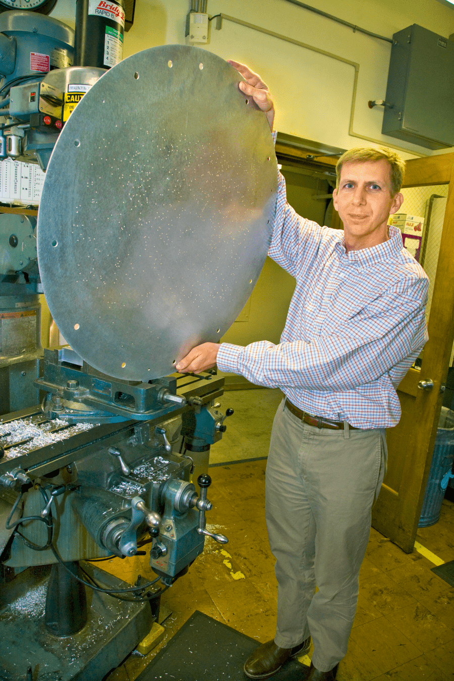
credits: LBL

credits: Thomas Nash
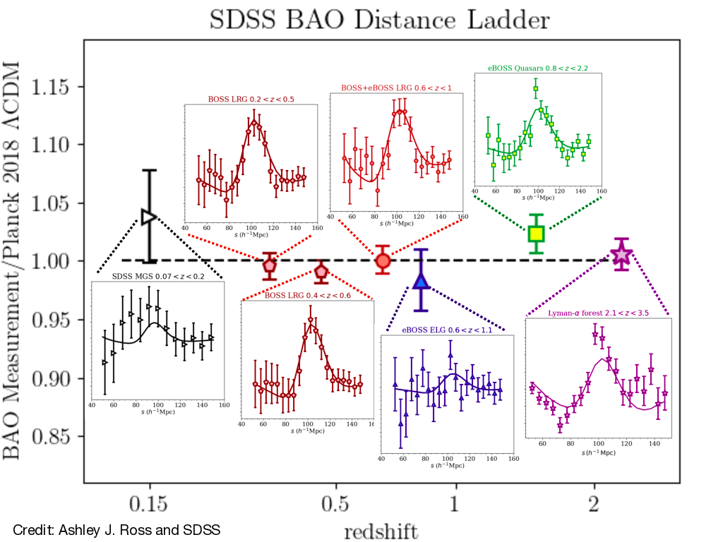
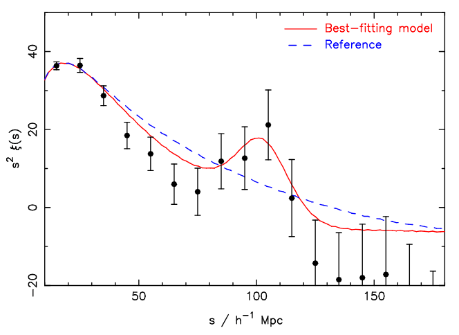
2dFGRS, SDSS: first BAO detection!
- In 2005, first evidence for Baryon Acoustic Oscillations
- Standard ruler to probe the expansion history of the Universe
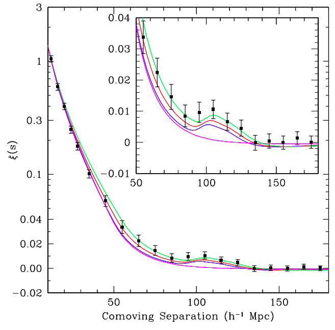
SDSS - 47k LRG \(0.16 < z < 0.47\)
Eisenstein et al. 2005
2dFGRS
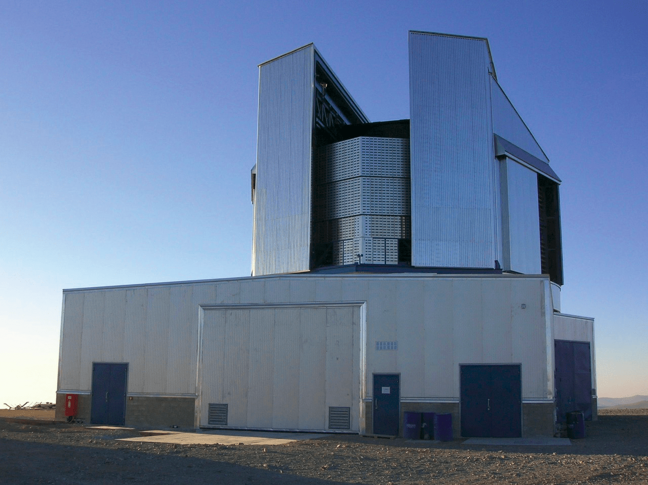
WiggleZ, BOSS/eBOSS: higher z
WiggleZ
- WiggleZ (2006-2011): upated 2dFGRS facility, 240k star-forming galaxies at intermediate redshifts (\(z \sim 0.6\))
- SDSS-III BOSS (2009-2014): 1.5M Luminous Red Galaxies and Quasars \((0.3 < z < 0.7)\)
- SDSS-IV eBOSS (2014-2020): +800k LRG, Emission Line Galaxies and Quasars up to \(z \sim 2\)
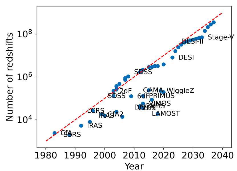
Large surveys
- made possible by multi-object spectroscopy
- high redshift (z > 0.5) surveys since 2005
Moore's law for spectroscopic surveys; Schlegel et al. 2022
Euclid
10 years = \(10 \times \)
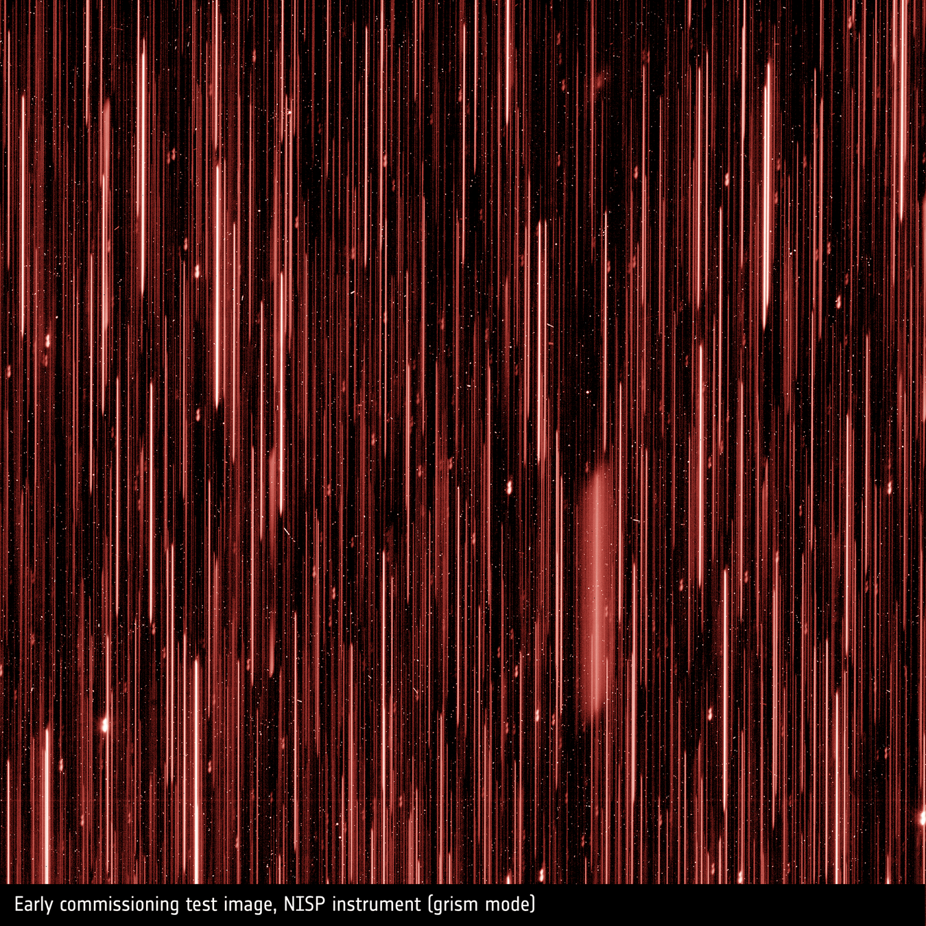
Stage IV experiments: Euclid
2023 - 2029: 35M H\(\alpha\) emitters at \(0.7 < z < 1.8\) over \(14 000 \; \mathrm{deg}²\)
Slitless spectroscopy with NISP: disperses the entire field-of-view:
- all spectra at once, no moving parts
- no need for target selection
- but difficult to deal with spectra overlap, noise subtraction, etc.
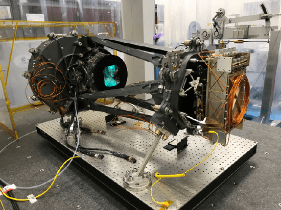
NISP instrument. Euclid consortium
ESA
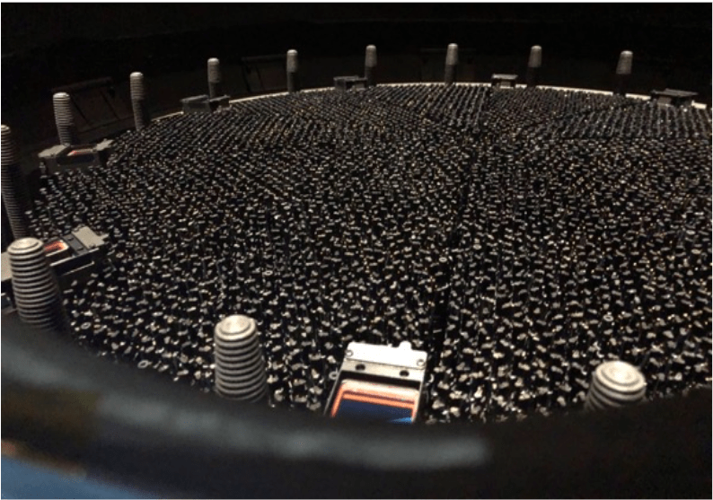
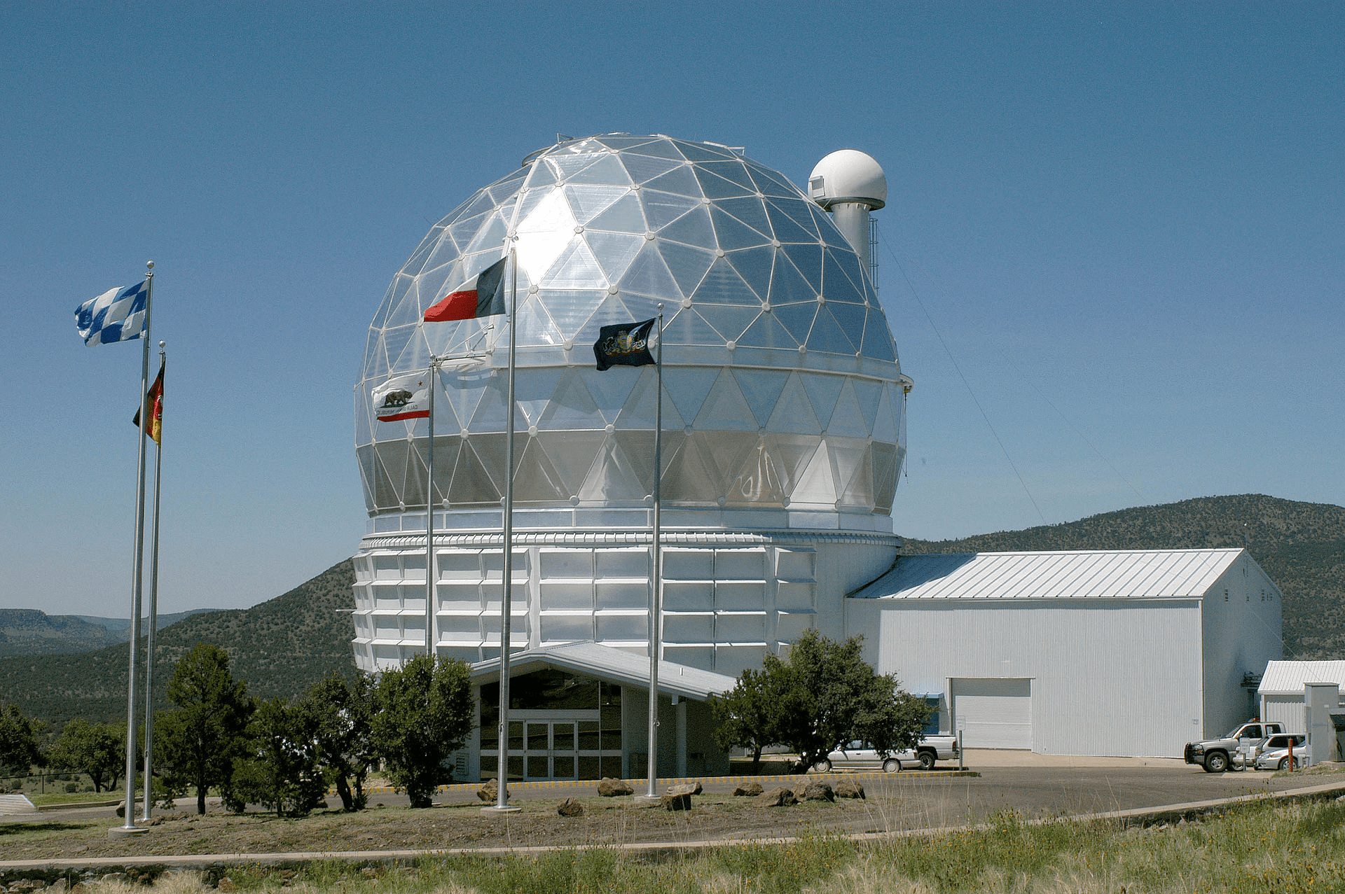
Stage IV experiments: DESI
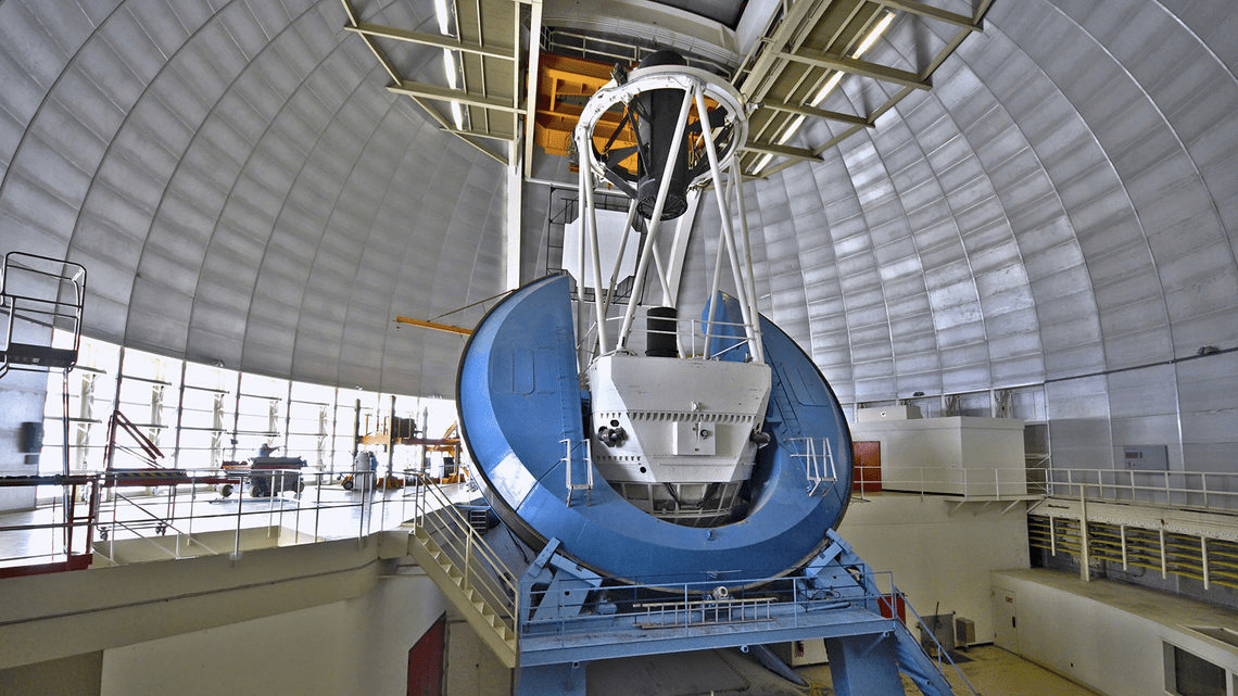
2021 - 2025: 40M redshifts at \(0 < z < 3\) over \(14 000 \; \mathrm{deg}²\)
Mayall Telescope at Kitt Peak, AZ
5000 robotically-positioned spectroscopic fibers
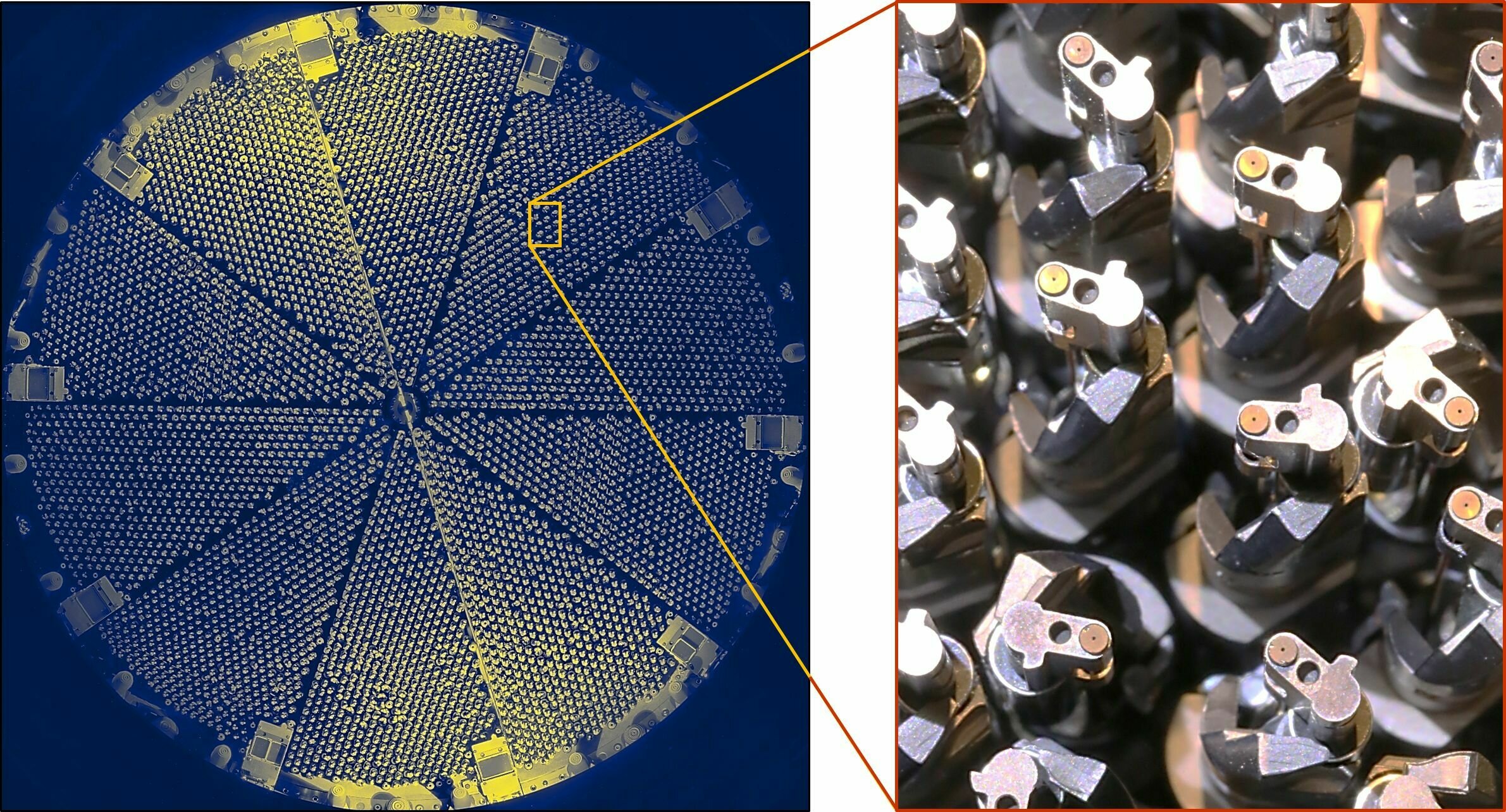
robotic positioners
Taken from Zhao et al. (2020)
DESI
Credit: NSF
Taken from Zhao et al. (2020)
DESI focal plane

DESI cosmological constraints
Measuring dark energy
\(\Lambda\)
2024
2025

DESI cosmological constraints
GR
Measuring dark energy
\(\Lambda\)
Testing general relativity
Taken from Zhao et al. (2020)
Other redshift surveys
- HETDEX (2017-2023): 1M (Lyman-\(\alpha\) emitting) galaxies, untargeted survey (R ∼ 800)
- 4MOST (2024-2029): 25M spectra \(15,000\;\mathrm{deg}^2\), Paranal Observatory, Chile
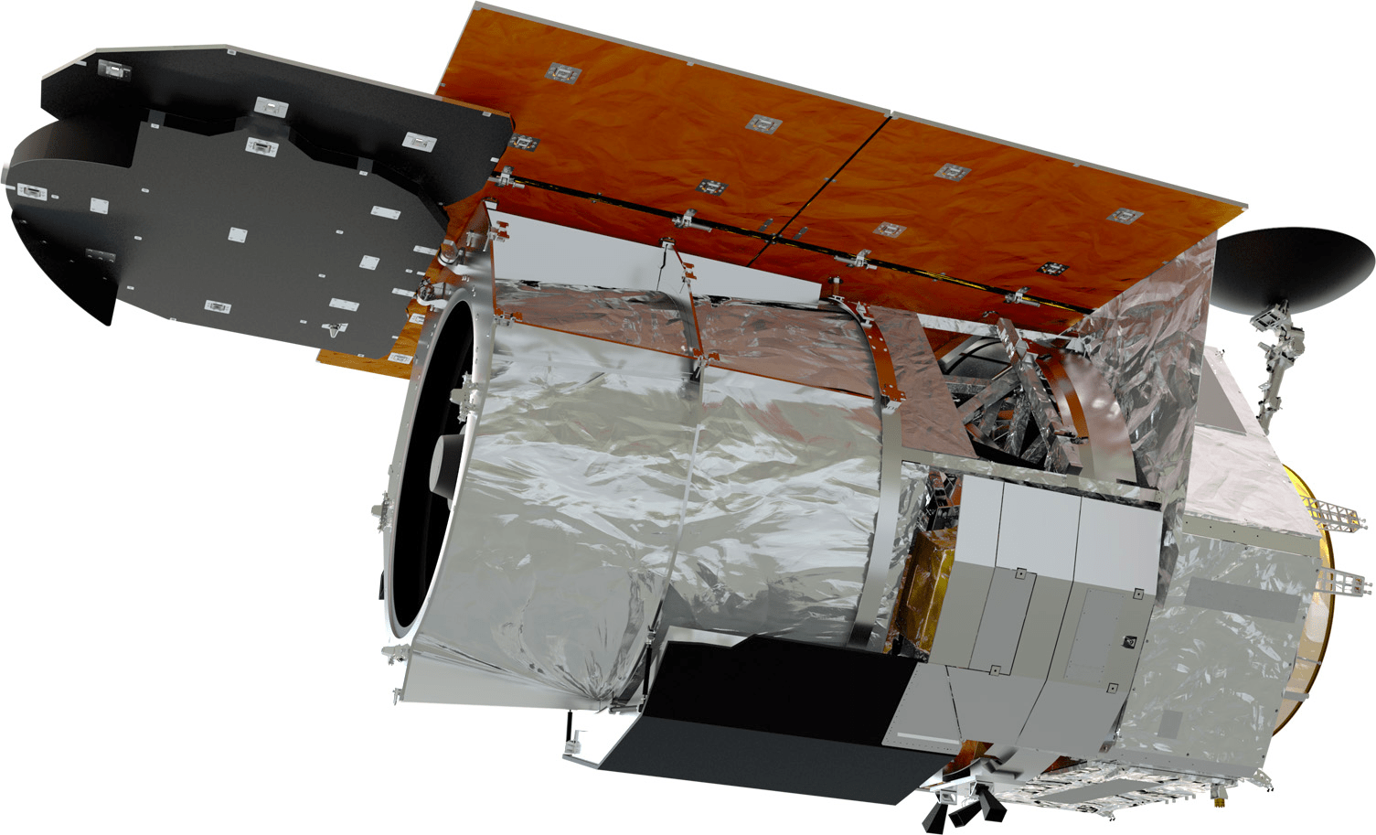
- Nancy-Grace-Roman / WFIRST (2025-2030): 20M H\(\alpha\) emitters (R = 70 − 140 and R = 450 − 850), slitless spectroscopy
Past and current surveys: take-aways
- Catalogs of galaxies have been built starting the 1920's (Hubble, Zwicky, etc.)
- Digitalization in the 1970's
- Redshift surveys as early as 1980's (CfA) revealed cosmic structures (walls, filaments). But it was slow...
- In the 90's, first evidence for \(\Omega_\mathrm{m} < 1\)
- >90's, multi-object spectroscopy allowed 100-1000 spectra to be measured at once: a revolution in survey speed!
- Big names: 2dFGRS, SDSS, DESI, Euclid...
- First evidence for BAO in 2005 (WiggleZ, SDSS), much progress since then!
- With DESI and Euclid: pin down dark energy, test modified gravity, primordial non-Gaussianity, etc.
how to extract cosmological information from our survey data?
Outline
- Past and current surveys
- Clustering observables
- Spectroscopic surveys and systematics
- Large-scale structure formation
- BAO and RSD theory models
- Current constraints
- Other clustering analyses
What do we measure?
We measure angular positions (right ascension (R.A.), declination
(Dec.)) and redshifts (\(z\)) of \(\mathcal{O}(10^6)\) galaxies.
What to do with this data?
SDSS data. Credits: EPFL
An example: ...
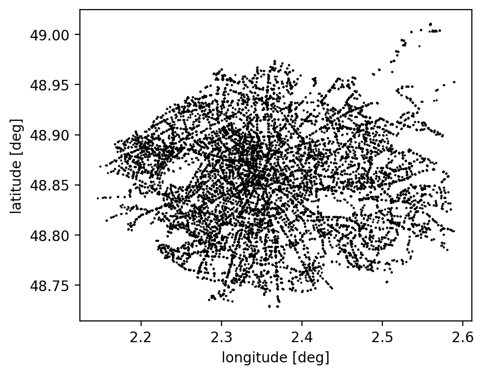
An example: Paris metro & bus stations
Credit to Etienne Burtin for the idea!
bois de Boulogne
bois de Vincennes
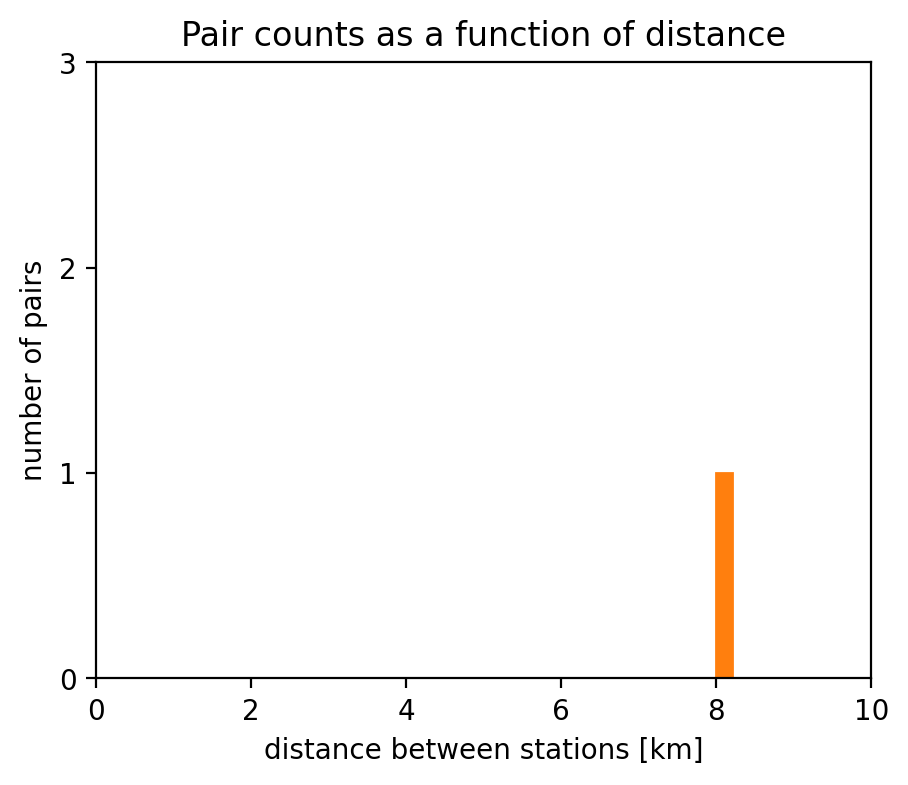
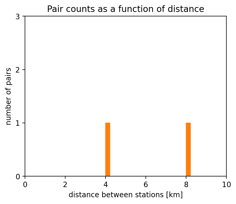
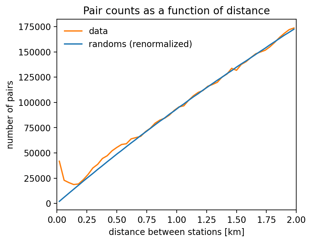
Counting pairs
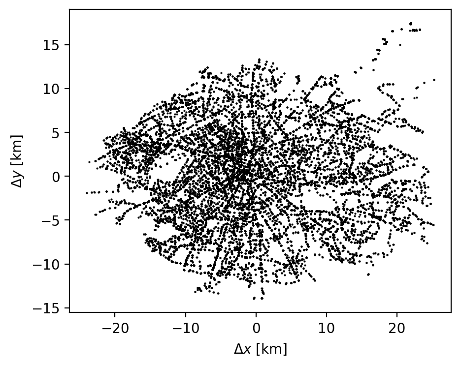
Counting pairs
Counting pairs
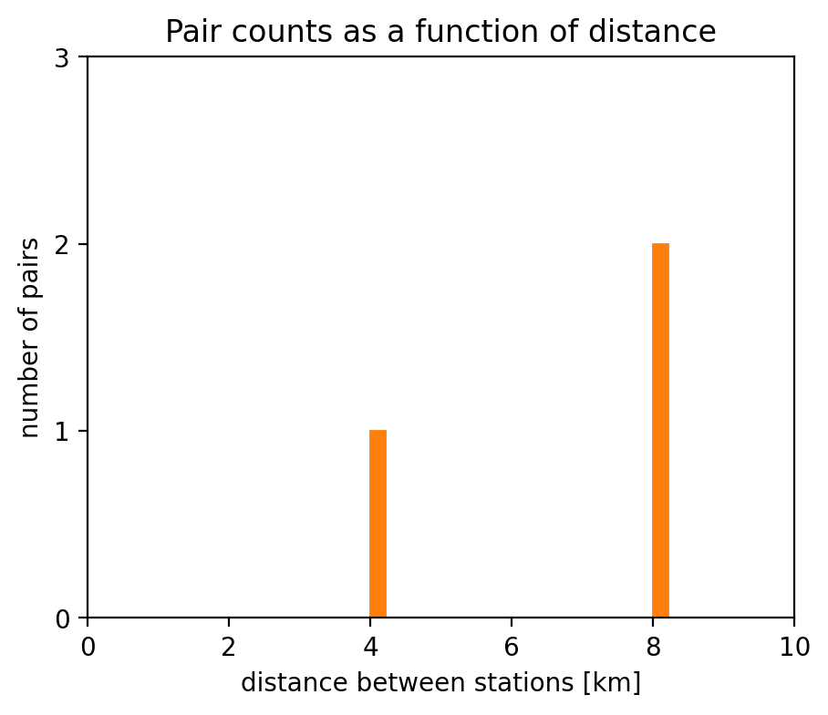
Counting pairs
edges = np.linspace(0., 2., 51)
# positions.shape = (N, 2)
# positions[:, 0] is x, positions[:, 1] is y

# Count pairs of points within a distance range
def pair_count_2d(positions, edges):
    counts = np.zeros(len(edges) - 1)
    for i in range(positions.shape[0]):
        for j in range(i + 1, positions.shape[0]):
            dx = positions[i, 0] - positions[j, 0]
            dy = positions[i, 1] - positions[j, 1]
            dist2 = dx * dx + dy * dy
            # Only count if within the maximum distance
            if dist2 < edges[-1]**2:
                # Find the index in the edges array
                idx = int((np.sqrt(dist2) - edges[0])\
                          / (edges[-1] - edges[0])\
                          * len(counts))
                counts[idx] += 1
    return counts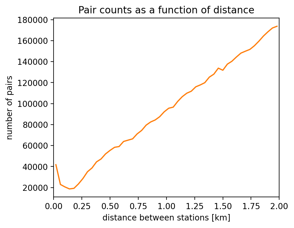
...a bit hard to interpret! Is the trend consistent with what one would expect is stations were distributed uniformly?
Randoms
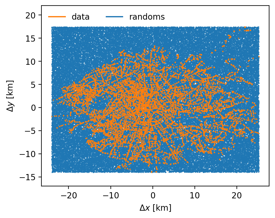
Let's just generate some uniformly-distributed "randoms"
Bonus question: what is ~the slope of this curve?
Randoms
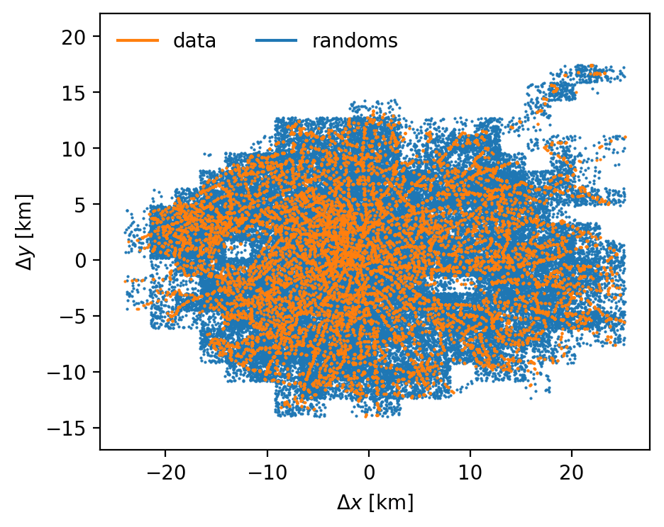
Let's imprint the footprint of Paris!
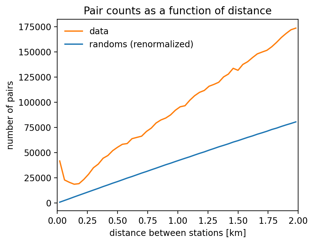
Randoms
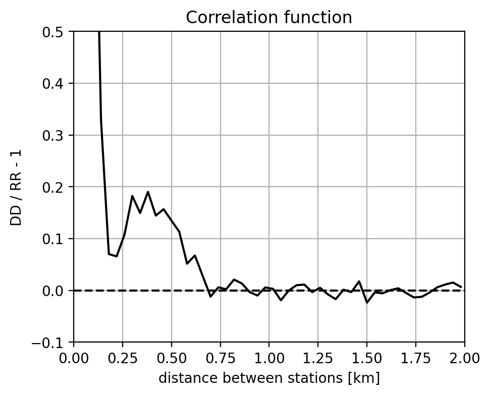
DD: data pair counts
RR: randoms pair counts
Randoms
DD: data pair counts
RR: randoms pair counts
clustered stations
characteristic scale of 0.4 km
A bit of formalism
\(n_\mathrm{g}(\mathbf{x}) = \bar{n}(\mathbf{x})\left[1 + \delta_\mathrm{g}(\mathbf{x}) \right]\) \(\delta_\mathrm{g}\) density contrast
Density of galaxies
A bit of formalism
\(n_\mathrm{g}(\mathbf{x}) = \bar{n}(\mathbf{x})\left[1 + \delta_\mathrm{g}(\mathbf{x}) \right]\) \(\delta_\mathrm{g}\) density contrast
Density of galaxies
Probability to find:
- one galaxy in \(dV_1\): \(dP_1 = \langle n_\mathrm{g}(\mathbf{x}_1) dV_1 \rangle = \bar{n}(\mathbf{x}_1) dV_1\)
A bit of formalism
Density of galaxies
Probability to find:
- one galaxy in \(dV_1\): \(dP_1 = \langle n_\mathrm{g}(\mathbf{x}_1) dV_1 \rangle = \bar{n}(\mathbf{x}_1) dV_1\)
- two galaxies in \(dV_1\) and \(dV_2\):
dP_{12} = \left\langle n_\mathrm{g}(\mathbf{x}_1) n_\mathrm{g}(\mathbf{x}_2) \right\rangle dV_1 dV_2 = \bar{n}(\mathbf{x}_1) \bar{n}(\mathbf{x}_2) \left[ 1 + \xi_\mathrm{gg}(\mathbf{x}_1, \mathbf{x}_2) \right] dV_1 dV_2
\(\xi_\mathrm{gg}(\mathbf{s}) = \left\langle \delta_\mathrm{g}(\mathbf{x}_1) \delta_\mathrm{g}(\mathbf{x}_1 + \mathbf{s}) \right\rangle\)
Covariance of the density contrast as a function of separation \(\mathbf{s}\)
Galaxy correlation function
Independent of position assuming spatial homogeneity.
\(n_\mathrm{g}(\mathbf{x}) = \bar{n}(\mathbf{x})\left[1 + \delta_\mathrm{g}(\mathbf{x}) \right]\) \(\delta_\mathrm{g}\) density contrast
Fiducial coordinates
Wait! What is \(\mathbf{x}\)? I thought that in the catalog we had R.A., Dec., z?
Fiducial coordinates
We use a fiducial cosmology to convert \(z\) to distance
\orange{D_c(z)} = \int_0^z \frac{c dz^\prime}{\green{H(z^\prime)}} \qquad \text{with} \qquad \green{H(z)} = \purple{H_0} \sqrt{\blue{\Omega_\mathrm{m}} (1 + z)^3 + 1 - \Omega_\mathrm{m}}
Distance in \(\mathrm{Mpc}/h\) units: only need to assume a fiducial \(\Omega_\mathrm{m}\)
Two angles on the sky (R.A., Dec.), and distance
\(\Rightarrow\) fiducial cartesian comoving coordinates \(\mathbf{x}\)
Note for later: include this in the theory model!
comoving radial distance
Hubble rate
matter density
Hubble parameter \(H_0 = 100\;h\;\mathrm{km}/\mathrm{s}/\mathrm{Mpc}\)
Fiducial coordinates
We use a fiducial cosmology to convert \(z\) to distance
Distance in \(\mathrm{Mpc}/h\) units: only need to assume a fiducial \(\Omega_\mathrm{m}\)
Two angles on the sky (R.A., Dec.), and distance
\(\Rightarrow\) fiducial cartesian comoving coordinates \(\mathbf{x}\)
Note for later: include this in the theory model!
comoving radial distance
Hubble rate
matter density
Hubble parameter \(H_0 = 100\;h\;\mathrm{km}/\mathrm{s}/\mathrm{Mpc}\)
\orange{D_c(z)} = \int_0^z \frac{c dz^\prime}{\green{H(z^\prime)}} \qquad \text{with} \qquad \green{H(z)} = \purple{H_0} \sqrt{\blue{\Omega_\mathrm{m}} (1 + z)^3 + 1 - \Omega_\mathrm{m}}
(Isotropic) correlation function
separation between galaxies
correlation function
excess probability that 2 galaxies are close
\(<0\) as \(\int d^3s \xi(s) = 0\)
excess probability that 2 galaxies are close
Power spectrum
Fourier transform of the density contrast \(\delta_\mathrm{g}(\mathbf{x})\)
\delta_\mathrm{g}(\mathbf{k}) = \int d^3x \, \delta_\mathrm{g}(\mathbf{x}) \, e^{i \mathbf{k} \cdot \mathbf{x}}
\((2\pi)^3 \delta_D^{(3)}(\mathbf{k} + \mathbf{k}') P_\mathrm{gg}(\mathbf{k}) = \langle \delta_\mathrm{g}(\mathbf{k}) \delta_\mathrm{g}(\mathbf{k}') \rangle\)
Galaxy power spectrum
- Dirac \(\delta_D^{(3)}(\mathbf{k} + \mathbf{k}')\) comes from homogeneity
Power spectrum
Fourier transform of the density contrast \(\delta_g(\mathbf{x})\)
Galaxy power spectrum
- Dirac \(\delta_D^{(3)}(\mathbf{k} + \mathbf{k}')\) comes from homogeneity
- \(\xi_\mathrm{gg}(\mathbf{s})\) and \(P_\mathrm{gg}(\mathbf{k})\) are Fourier transform pairs:
Early time/large scales, \(\delta\) follows Gaussian statistics: fully described by 2-point function.
P_\mathrm{gg}(\mathbf{k}) = \int d^3 s \, \xi_\mathrm{gg}(\mathbf{s}) \, e^{i \mathbf{k} \cdot \mathbf{s}}
\delta_\mathrm{g}(\mathbf{k}) = \int d^3x \, \delta_\mathrm{g}(\mathbf{x}) \, e^{i \mathbf{k} \cdot \mathbf{x}}
\((2\pi)^3 \delta_D^{(3)}(\mathbf{k} + \mathbf{k}') P_\mathrm{gg}(\mathbf{k}) = \langle \delta_\mathrm{g}(\mathbf{k}) \delta_\mathrm{g}(\mathbf{k}') \rangle\)
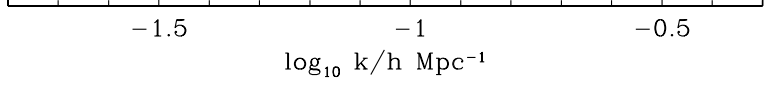
(Isotropic) power spectrum
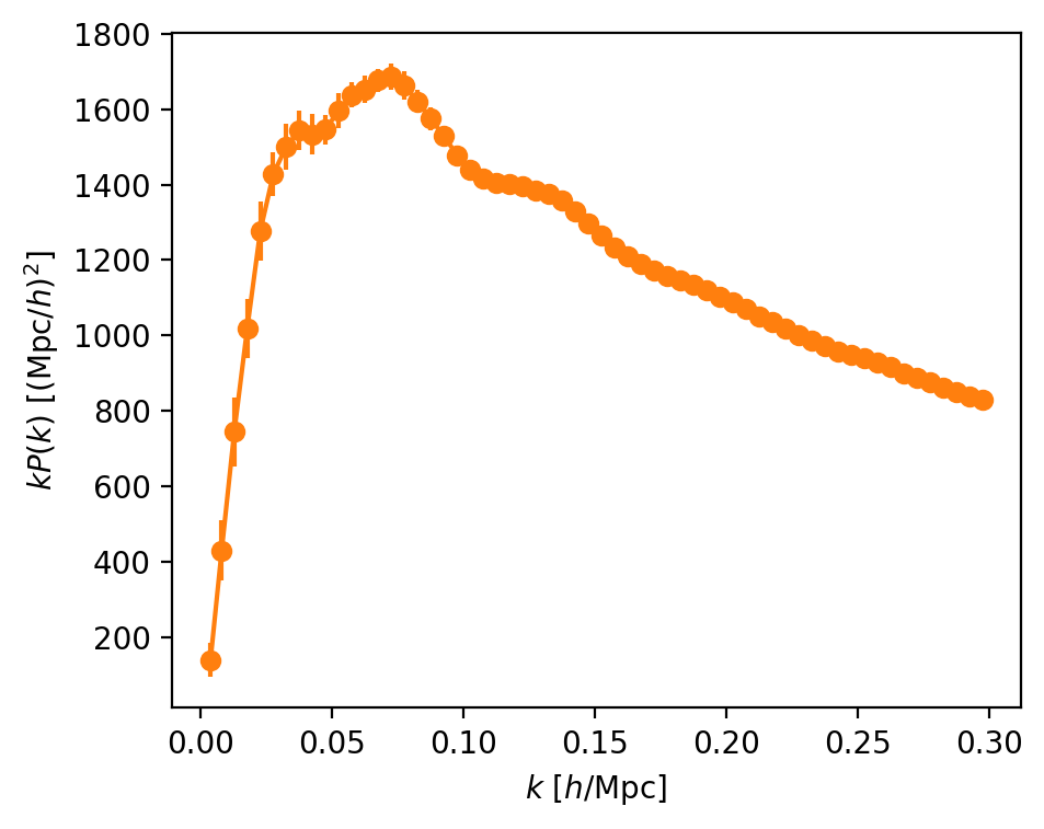
power spectrum
wavenumber
small scales
large scales
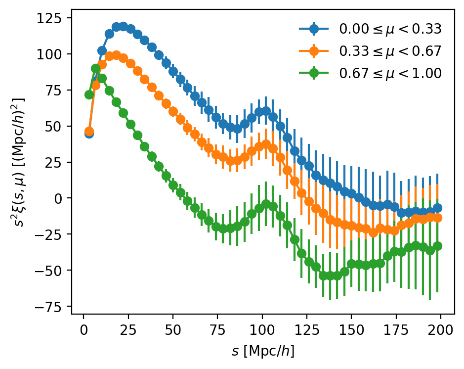
Anisotropic clustering
In practice, the clustering amplitude does not only depend on the separation \(|\mathbf{s}|\) or wavenumber \(|\mathbf{k}|\)...
But also on the direction of \(\mathbf{s}\) and \(\mathbf{k}\)
Q: Wait, isn't the Universe homogeneous and isotropic?
Anisotropic clustering
In practice, the clustering amplitude does not only depend on the separation \(|\mathbf{s}|\) or wavenumber \(|\mathbf{k}|\)...
But also on the direction of \(\mathbf{s}\) and \(\mathbf{k}\)
Q: Wait, isn't the Universe homogeneous and isotropic?
In practice, the clustering amplitude does not only depend on the separation \(|\mathbf{s}|\) or wavenumber \(|\mathbf{k}|\)...
But also on the direction of \(\mathbf{s}\) and \(\mathbf{k}\)
direction of a galaxy = line-of-sight
Anisotropic clustering
In practice, the clustering amplitude does not only depend on the separation \(|\mathbf{s}|\) or wavenumber \(|\mathbf{k}|\)...
But also on the direction of \(\mathbf{s}\) and \(\mathbf{k}\)
"midpoint" line-of-sight
\(\mathbf{s} = \mathbf{x}_2 - \mathbf{x}_1\) separation
We usually call \(\mu = \hat{\mathbf{s}} \cdot \hat{\mathbf{\eta}}\) the cosine angle between the separation vector \(\mathbf{s}\) and the line-of-sight \(\hat{\mathbf{\eta}}\)
Similarly: \(\mu = \hat{\mathbf{k}} \cdot \hat{\mathbf{\eta}}\)
\(\hat{\eta} = \widehat{\mathbf{x}_1 + \mathbf{x}_2}\)
\(\mathbf{x}_1\)
\(\mathbf{x}_2\)
\(\mu\)
Anisotropic clustering
Anisotropic clustering
Anisotropic clustering
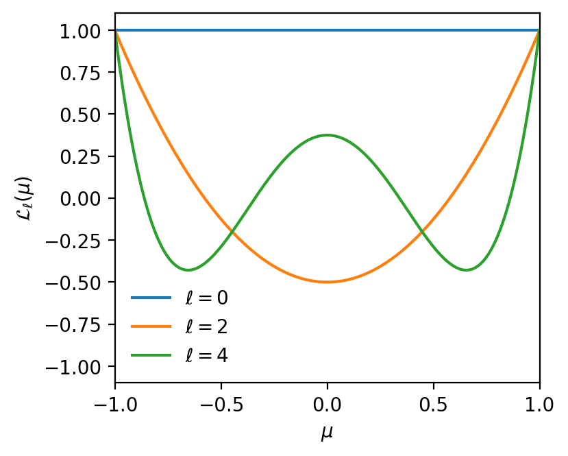
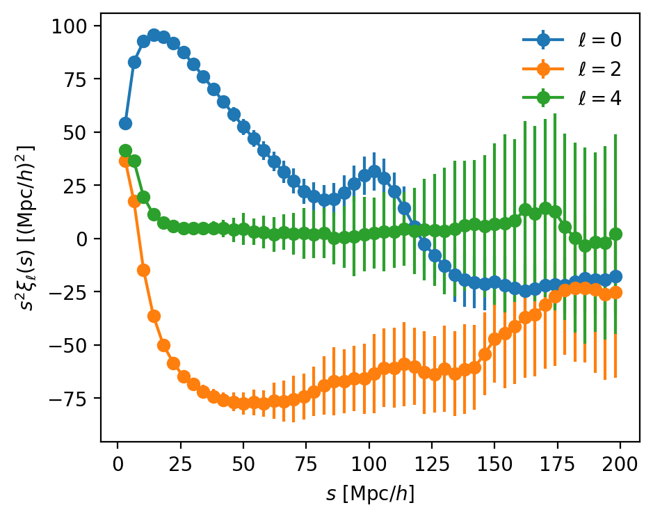
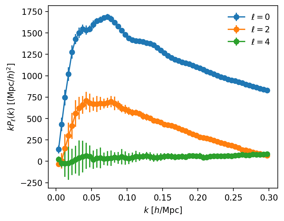
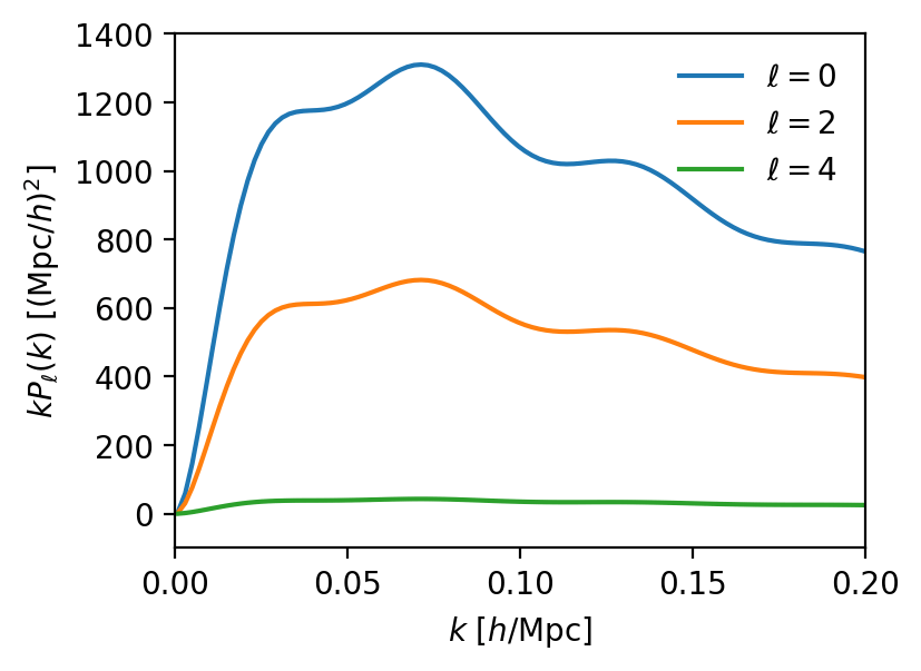
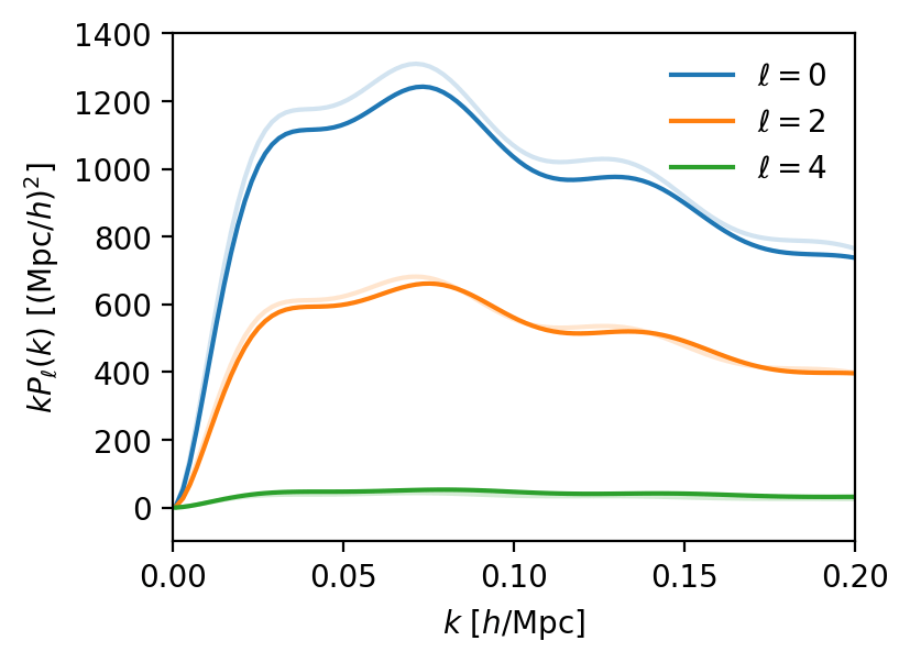
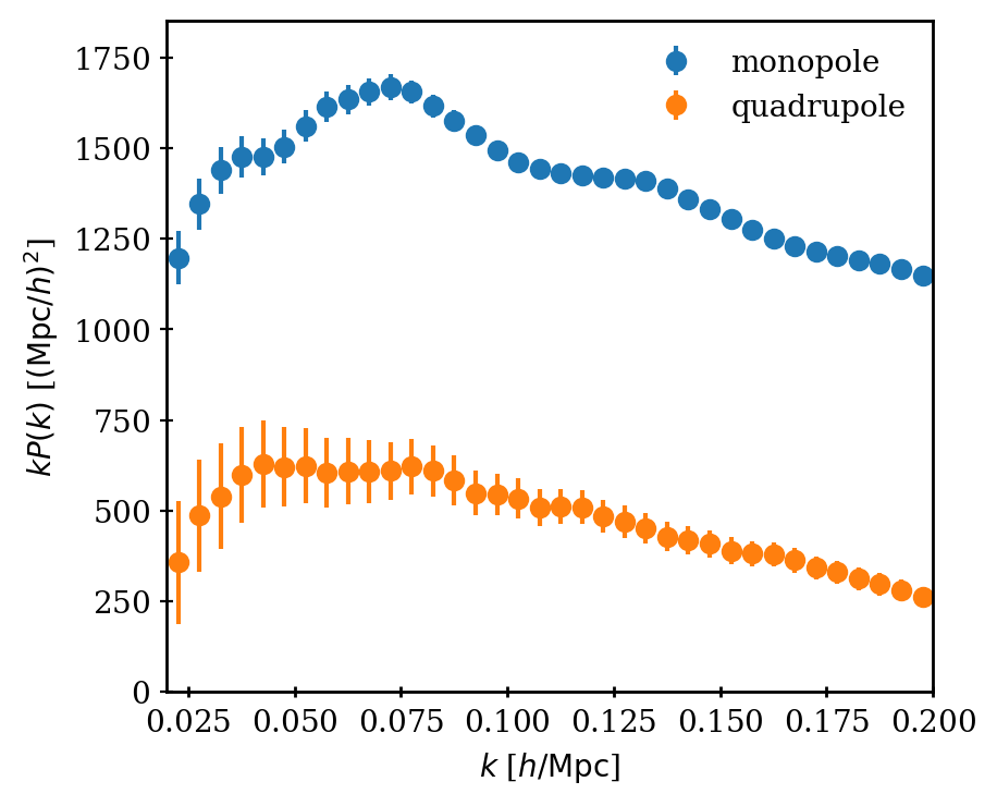
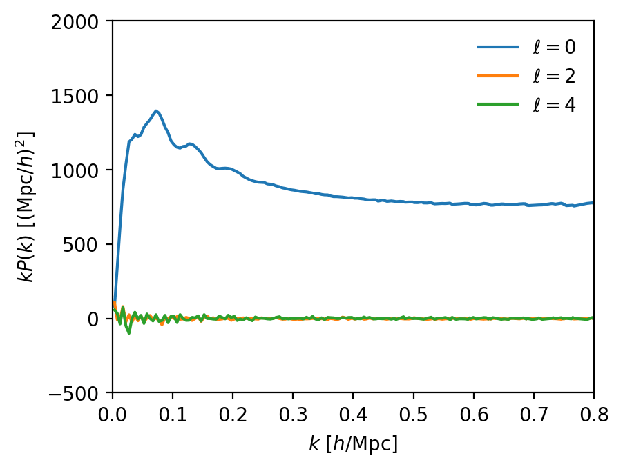
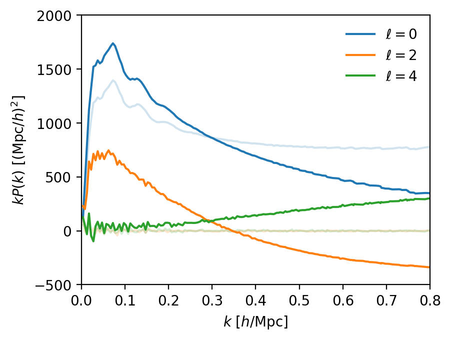
In practice, rather than binning in \(\mu\), we prefer to measure Legendre multipoles \(\xi_\ell(s)\) and \(P_\ell(k)\), typically \(0 \leq \ell \leq 4\)
\xi(s, \mu) = \sum_{\ell = 0}^{+\infty} \xi_{\ell}(s) \orange{\mathcal{L}_{\ell}(\mu)}
\quad \& \quad
P(k, \mu) = \sum_{\ell = 0}^{+\infty} P_{\ell}(k) \orange{\mathcal{L}_{\ell}(\mu)}
\xi_{\ell}(s) = \frac{2 \ell + 1}{2} \int_{-1}^{1}d\mu \xi(s, \mu) \orange{\mathcal{L}_{\ell}(\mu)}
\quad \& \quad
P_{\ell}(k) = \frac{2 \ell + 1}{2} \int_{-1}^{1}d\mu P(k, \mu) \orange{\mathcal{L}_{\ell}(\mu)}
Legendre polynomial
Anisotropic clustering
In practice, rather than binning in \(\mu\), we prefer to measure Legendre multipoles \(\xi_\ell(s)\) and \(P_\ell(k)\), typically \(0 \leq \ell \leq 4\)
\xi(s, \mu) = \sum_{\ell = 0}^{+\infty} \xi_{\ell}(s) \orange{\mathcal{L}_{\ell}(\mu)}
\quad \& \quad
P(k, \mu) = \sum_{\ell = 0}^{+\infty} P_{\ell}(k) \orange{\mathcal{L}_{\ell}(\mu)}
\xi_{\ell}(s) = \frac{2 \ell + 1}{2} \int_{-1}^{1}d\mu \xi(s, \mu) \orange{\mathcal{L}_{\ell}(\mu)}
\quad \& \quad
P_{\ell}(k) = \frac{2 \ell + 1}{2} \int_{-1}^{1}d\mu P(k, \mu) \orange{\mathcal{L}_{\ell}(\mu)}
Then one can show that \(\xi_\ell(s)\) and \(P_\ell(k)\) are related through a Hankel transform:
P_\ell(k) = 4\pi i^\ell \int s^2 ds \orange{j_\ell(k s)} \xi_\ell(s) \quad \& \quad \xi_\ell(s) = \frac{(-i)^\ell}{2\pi^2} \int k^2 dk \orange{j_\ell(k s)} P_\ell(k)
spherical Bessel function
Anisotropic clustering
How to estimate \(\xi_\ell(s)\) and \(P_\ell(k)\) from galaxy catalogs?
Clustering catalogs
Catalog of particles (R.A., Dec., \(z\)) that randomly sample the survey selection function \(\bar{n}\) (i.e. where we carried out observations).
Usually \(>20\times\) denser than the data catalogs, to reduce sampling noise.
"Randoms"
Catalog of galaxies (R.A., Dec., \(z\), optionally weights)
"Data"
Correlation function estimators
Let \(XY(\mathbf{s})\) be the (normalized, weighted) number of pairs of objects from catalogs \(X, Y\) as a function of separation \(\mathrm{s}\)
\(\hat{\xi}(\mathbf{s}) = \frac{DD(\mathbf{s})}{RR(\mathbf{s})} − 1\) minimally biased but large variance
Natural estimator
\(\hat{\xi}(\mathbf{s}) = \frac{DD(\mathbf{s})}{DR(\mathbf{s})} − 1\) biased and not minimal variance
Davis and Peebles 1983 estimator
\(\hat{\xi}(\mathbf{s}) = \frac{DD(\mathbf{s}) RR(\mathbf{s})}{DR(\mathbf{s})^2} − 1\) minimal variance but biased
Hamilton 1993 estimator
Correlation function estimators
\(\hat{\xi}(\mathbf{s}) = \frac{DD(\mathbf{s})}{RR(\mathbf{s})} − 1\) minimally biased but large variance
Natural estimator
\(\hat{\xi}(\mathbf{s}) = \frac{DD(\mathbf{s})}{DR(\mathbf{s})} − 1\) biased and not minimal variance
Davis and Peebles 1983 estimator
\(\hat{\xi}(\mathbf{s}) = \frac{DD(\mathbf{s}) RR(\mathbf{s})}{DR(\mathbf{s})^2} − 1\) minimal variance but biased
Hamilton 1993 estimator
\(\hat{\xi}(\mathbf{s}) = \frac{DD(\mathbf{s}) - 2DR(\mathbf{s}) + RR(\mathbf{s})}{RR(\mathbf{s})}\) minimally biased, minimal variance
Landy-Szalay 1993 estimator
Let \(XY(\mathbf{s})\) be the (normalized, weighted) number of pairs of objects from catalogs \(X, Y\) as a function of separation \(\mathrm{s}\)
Power spectrum estimator
\(F(\mathbf{x}) = n_\mathrm{g}(\mathbf{x}) − \bar{n}(\mathbf{x})\)
Density fluctuations
Yamamoto 2006 estimator
\hat{P}_{\ell}(k) = \frac{2\ell + 1}{A N_k} \sum_{\mathbf{k} \in k-\mathrm{bin}} F_{\ell}^{\star}(\mathbf{k}) F_{0}(\mathbf{k}) - P_{\ell}^{\mathrm{noise}}(k)
F_{\ell}(\mathbf{k}) = \sum_{\mathbf{x}} e^{i \mathbf{k} \cdot \mathbf{x}} F(\mathbf{x}) \mathcal{L}_\ell(\mathbf{\hat{k}} \cdot \mathbf{\hat{x}})
\(P_\ell^\mathrm{noise}(k) \simeq \delta_{\ell 0}^{K} \bar{n}^{-1}\): shot noise due to finite number of galaxies
number of \(\mathbf{k}\)-modes in the bin
A = \sum_\mathbf{x} \bar{n}^{2}(\mathbf{x})
normalisation
computed with Fast Fourier Transforms
\(F\) painted on a mesh (\(\Rightarrow\) aliasing effects)
Power spectrum estimator
\(F(\mathbf{x}) = n_\mathrm{g}(\mathbf{x}) − \bar{n}(\mathbf{x})\)
Density fluctuations
Yamamoto 2006 estimator
\hat{P}_{\ell}(k) = \frac{2\ell + 1}{A N_k} \sum_{\mathbf{k} \in k-\mathrm{bin}} F_{\ell}^{\star}(\mathbf{k}) F_{0}(\mathbf{k}) - P_{\ell}^{\mathrm{noise}}(k)
F_{\ell}(\mathbf{k}) = \sum_{\mathbf{x}} V_\mathrm{cell} e^{i \mathbf{k} \cdot \mathbf{x}} F(\mathbf{x}) \mathcal{L}_\ell(\mathbf{\hat{k}} \cdot \mathbf{\hat{x}})
\(P_\ell^\mathrm{noise}(k) \simeq \delta_{\ell 0}^{K} \bar{n}^{-1}\): shot noise due to finite number of galaxies
number of \(\mathbf{k}\)-modes in the bin
A = \sum_\mathbf{x} V_\mathrm{cell} \bar{n}^{2}(\mathbf{x})
normalisation
computed with Fast Fourier Transforms
Window function effect
Survey has finite size: window function effect
- correlation function: already corrected for by the \(RR(s, \mu)\) term in the denominator
- power spectrum: to be deconvolved, or included in power spectrum model: matrix multiplication (e.g. Beutler and McDonald 2021) \(W_{\alpha\beta} = d\langle \hat{P}_\alpha \rangle / d P_\beta\)
- other effects: wide-angle, integral constraints (Beutler et al. 2019; de Mattia and Ruhlmann-Kleider 2019)
- "alternative": Optimal Quadratic Estimator (e.g. Philcox et al. 2024)
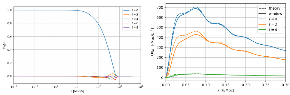
For a \(6\; \mathrm{Gpc}/h\) box
Measurement covariance
Power spectrum covariance is, using Wick’s theorem (Gaussian field):
\sigma(P(k))^2 \simeq \frac{2 (2\pi)^{3}}{A^{2}\Delta V_{k}} \int d^{3} x \bar{n}(\mathbf{x})^{4} \left[P(\mathbf{k}) + \frac{1}{\bar{n}(\mathbf{x})}\right]^{2}
minimizing variance: FKP (Feldman et al. 1994) weights
\(w_\mathrm{FKP} = 1/ [1 + \bar{n}(z)P_0)]\) applied to galaxies (and randoms)
e.g. Grieb et al. 2015
Measurement covariance
Power spectrum covariance is, using Wick’s theorem (Gaussian field):
- covariance matrix typically estimated from mocks: fast simulations of the galaxy density field, including survey selection function
- noise in the covariance matrix: noise in the cosmological measurement. Artificially enlarge error bars (Hartlap et al. 2007; Percival et al. 2014; Percival et al. 2022)
- accurate analytic estimations are developed (e.g. Lin et al. 2018, Wadekar et al. 2019)
\sigma(P(k))^2 \simeq \frac{2 (2\pi)^{3}}{A^{2}\Delta V_{k}} \int d^{3} x \bar{n}(\mathbf{x})^{4} \left[P(\mathbf{k}) + \frac{1}{\bar{n}(\mathbf{x})}\right]^{2}
minimizing variance: FKP (Feldman et al. 1994) weights
\(w_\mathrm{FKP} = 1/ [1 + \bar{n}(z)P_0)]\) applied to galaxies (and randoms)
e.g. Grieb et al. 2015
Measurement covariance
In the uniform \(\bar{n}\) limit:
- larger survey volume: \(\mathrm{error} \propto 1/\sqrt{\blue{V_s}}\)
- higher density: \(\mathrm{error} \propto 1/\orange{\bar{n}}\) when in the shot-noise dominated regime \(\bar{n} \ll 1/P_0\)
Two leverages to minimize variance (= higher measurement precision):
Credit: DESI
\sigma(P(k))^2 \simeq \frac{2 (2\pi)^{3}}{\Delta V_{k} \blue{V_{s}}} \left[P(k) + \frac{1}{\orange{\bar{n}}}\right]^{2}
Clustering observables: take-aways
- The clustering of galaxies can be probed through the correlation function \(\xi(\mathbf{s})\) or power spectrum \(P(\mathbf{k})\) (FT pair)
- Contain all information on \(\delta_\mathrm{g}\) if it is Gaussian (large scales)
- Anisotropic measurements: dependence on the (cosine) angle w.r.t. the line-of-sight \(\mu\); expansion in multipoles
- Various estimators exist; beware of the effect of the survey selection function!
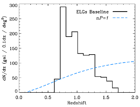
- Measurement uncertainty is \(\propto 1/\sqrt{V}\) and, in the shot noise dominated regime \(1/\bar{n}\) \(\Rightarrow\) \(\bar{n} P = 1\) criterion
how to carry out galaxy redshift surveys?
(disclaimer: with a focus on DESI!)
Clustering observables: take-aways
- The clustering of galaxies can be probed through the correlation function \(\xi(\mathbf{s})\) or power spectrum \(P(\mathbf{k})\) (FT pair)
- Contain all information on \(\delta_\mathrm{g}\) if it is Gaussian (large scales)
- Anisotropic measurements: dependence on the (cosine) angle w.r.t. the line-of-sight \(\mu\); expansion in multipoles
- Various estimators exist; beware of the effect of the survey selection function!
- Measurement uncertainty is \(\propto 1/\sqrt{V}\) and, in the shot noise dominated regime \(\propto 1/\bar{n}\) \(\Rightarrow\) \(\bar{n} P = 1\) criterion
how to carry out galaxy redshift surveys?
(disclaimer: with a focus on DESI!)
Outline
- Past and current surveys
- Clustering observables
- Spectroscopic surveys and systematics
- Large-scale structure formation
- BAO and RSD theory models
- Current constraints
- Other clustering analyses
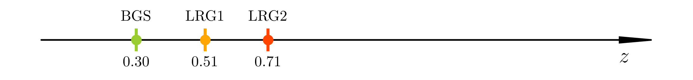
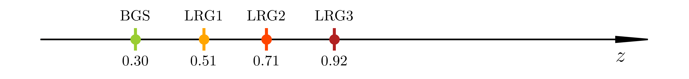
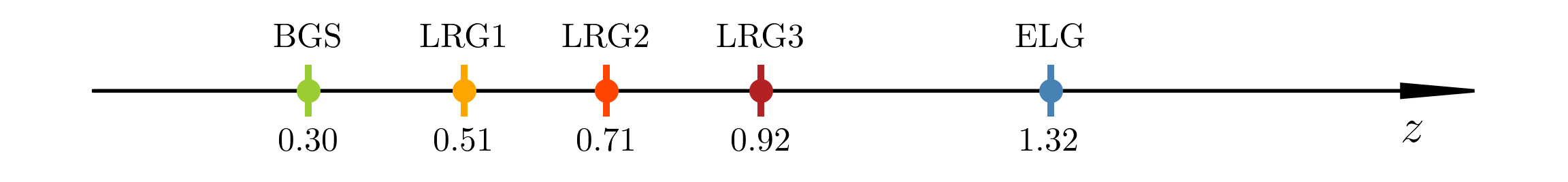
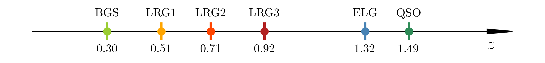
DESI Y5 galaxy samples
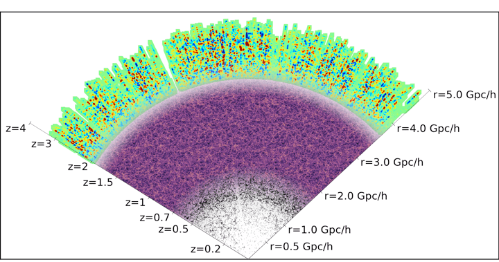
Bright Galaxies: 14M (SDSS: 600k)
0 < z < 0.4
LRG: 8M (SDSS: 1M)
0.4 < z < 1.1
ELG: 16M (SDSS: 200k)
0.6 < z < 1.6
QSO: 3M (SDSS: 500k)
Lya \(1.8 < z\)
Tracers \(0.8 < z < 2.1\)
Y5 (DR1-DR2-DR3) \(\sim 40\)M galaxy redshifts!
\(z = 0.4\)
\(z = 0.8\)
\(z = 0\)
\(z = 1.6\)
\(z = 2.0\)
\(z = 3.0\)
Spectroscopic galaxy surveys


imaging surveys (2014 - 2019) + WISE (IR)
target selection
spectroscopic observations
spectra and redshift measurements
- two steps: photometry and spectroscopy ⇒ selection effects
- catalog of angular positions \(\mathrm{R.A.}, \mathrm{Dec.}\) and redshifts \(z\)
Survey selection function
specify the survey selection function \(\bar{n}\) \(\Rightarrow\) account for systematic effects due to photometry/spectroscopy
Expected density without clustering = angular & radial footprint
Survey selection function \(\bar{n}\)
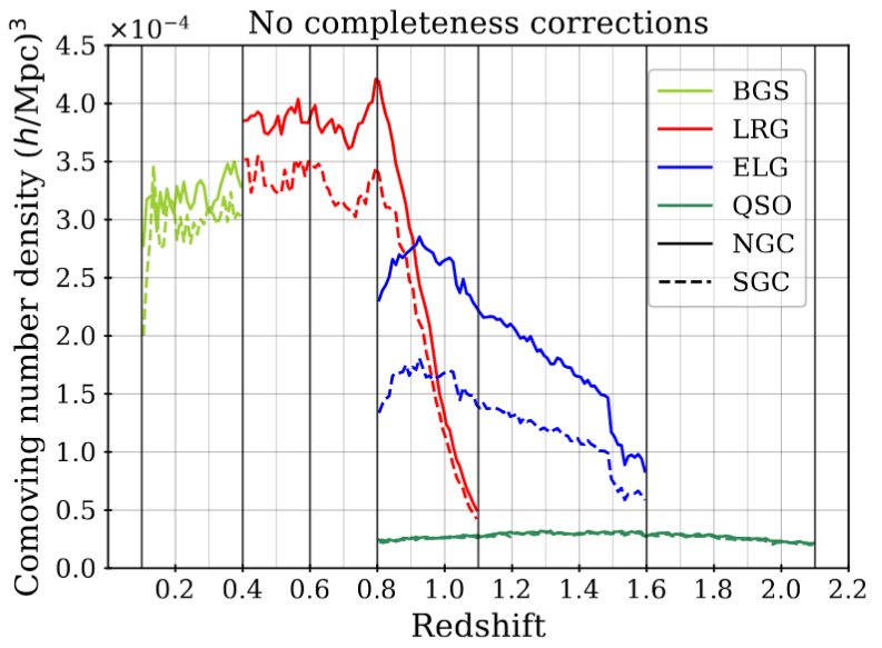
survey selection function \(\bar{n}\)
Taken from DESI Collaboration et al. 2024
Photometry
- photometric surveys: images of the sky, taken with different filters
- mainly characterized by their depth (magnitude corresponding to given probability of source detection), seeing (\(\in\) size of PSF)
- pipeline for source detection and source fitting (flux, shape, etc.)
- Legacy Surveys: https://www.legacysurvey.org/viewer
Taken from Zhao et al. (2020)
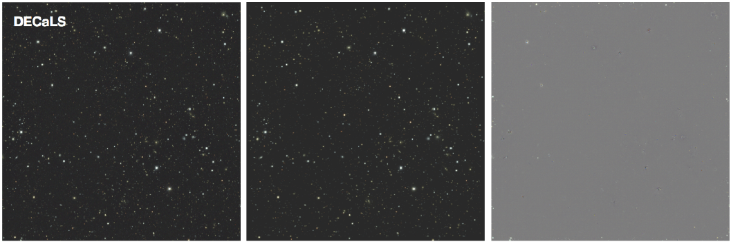
From left to right: data, model, residual. From Dey et al. (2019) (DECaLS DR8).
Target selection
- to obtain objects of certain class (luminous red galaxies, emission line galaxies, quasars...) in a redshift range
- typically with cuts in colour and magnitude
- usually, tradeoff between target density and purity
Taken from Zhao et al. (2020)
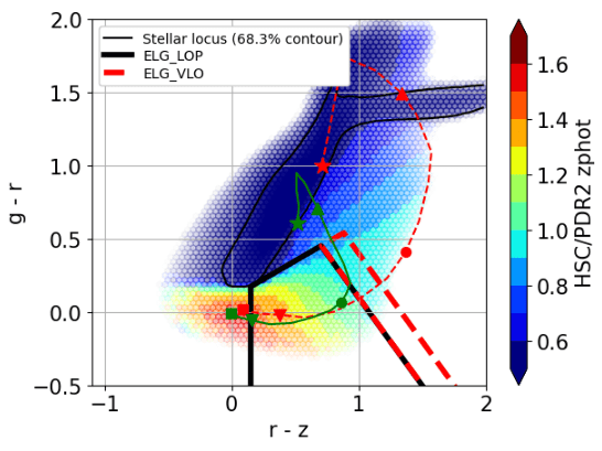
c) high-z
b) star / low-z rejection
d) [OII]
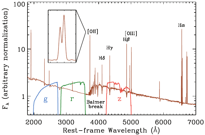
Left: taken from Raichoor et al. (2022). Right: taken from DESI Collaboration et al. (2016).
Photometric systematics
- veto masks in selection function n̄ for bright objects, (variable) stars, bad pixels...
-
target density varies with observational conditions: depth,
seeing, galaxy extinction, star density... to be modelled
Taken from Zhao et al. (2020)
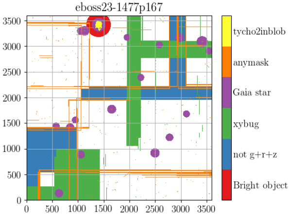
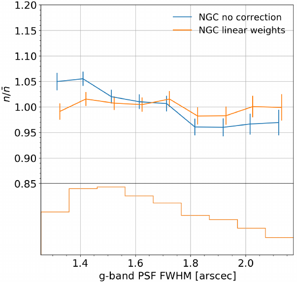
Left: masks on a legacypipe \(0.25^\circ × 0.25^\circ\) brick.
Taken from Raichoor et al. (2020).
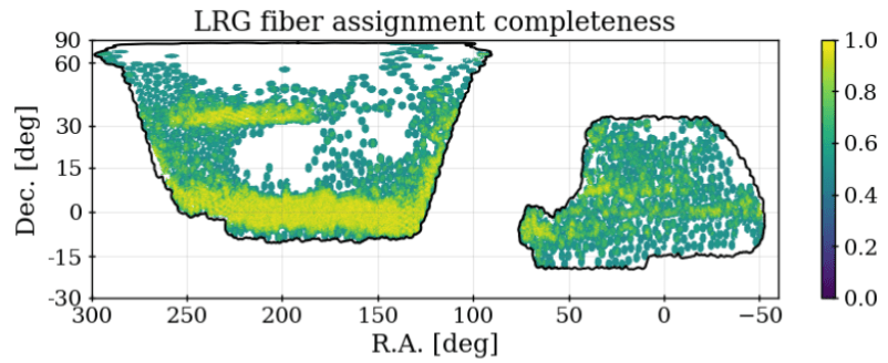
Fiber assignment
-
Fiber-fed spectrographs: fibers cannot be too close (e.g. 62'′ for SDSS) / "fixed density of fibers"
- SDSS-I < IV: hand-plugged fibers
- 2dFGRS, WiggleZ: fibers positioned by a robot
- SDSS V, DESI: robotic positioner for each fiber
Taken from Zhao et al. (2020)
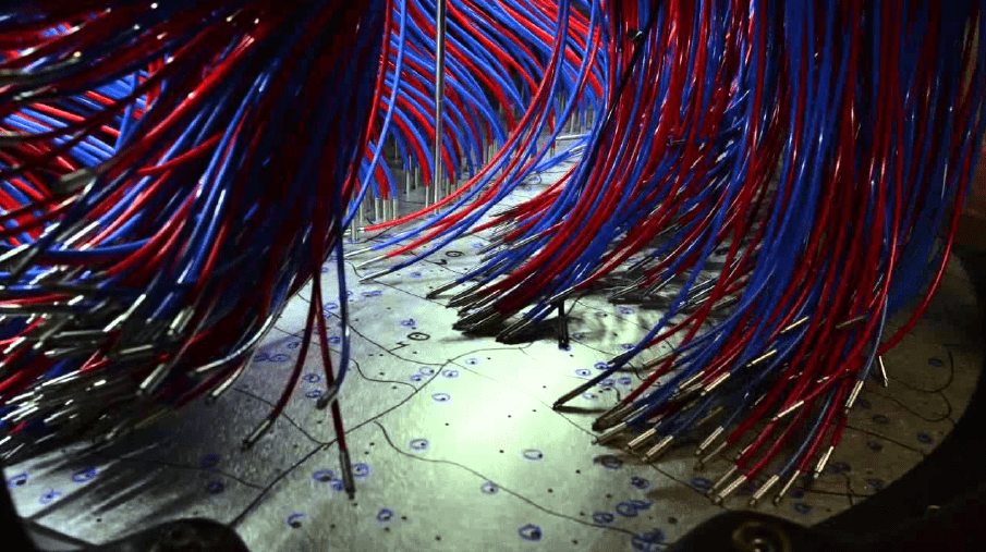
Credit: SDSS
Credit: DESI
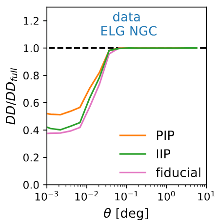
Fiber assignment
- density-dependent effect: correlates with clustering
Taken from Zhao et al. (2020)
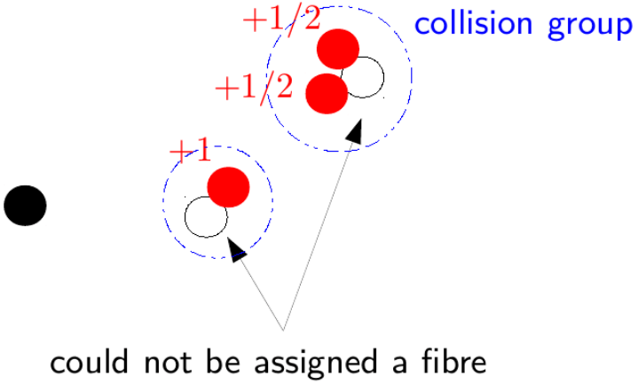
Individual galaxy weights not sufficient:
- pairwise inverse probability weights (PIP) (e.g. Bianchi and Percival 2017): rerun fiber assignment many times with different random seeds
- \(\theta\)-cut: remove all small scale angular pairs (e.g. Pinon et al. 2024)
\(0.05^\circ \simeq\) positioner patrol diameter
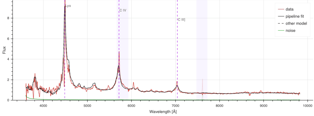
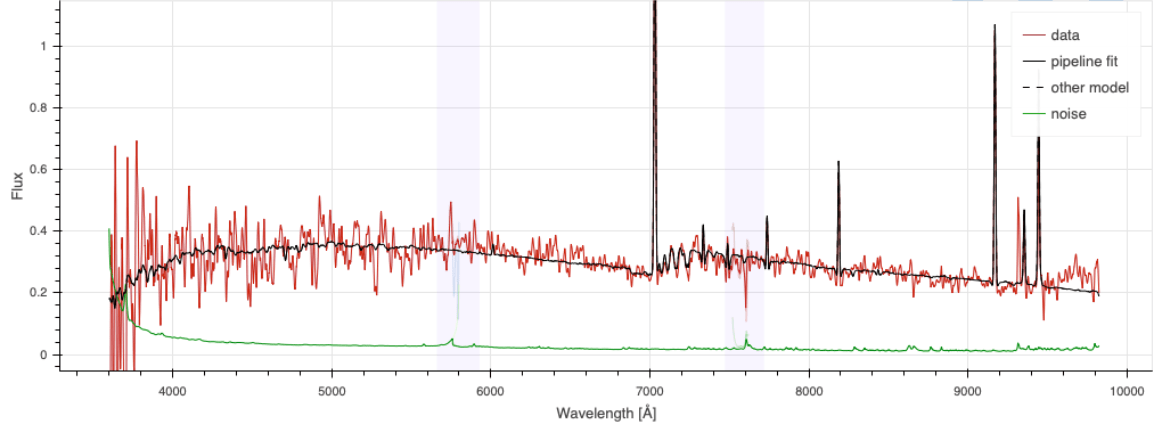
Spectroscopic measurements
Taken from Zhao et al. (2020)
- grims disperse light onto the focal plane
- reduction of 2D traces into 1D
- spectrum fit with a basis of archetypes / PCA templates
- criterion to select reliable redshifts
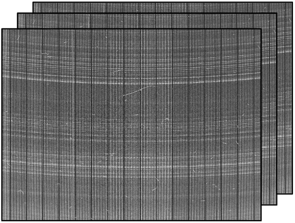
wavelength
fiber number
\(z = 2.1\) QSO
\(z = 0.9\) ELG
Ly\(\alpha\)
CIV
CIII
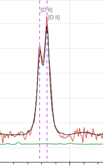
[OII] doublet at \(3727 \AA\) up to \(z = 1.6\)
[OII]
Ly\(\alpha\) at \(1216 \AA\) down to \(z = 2.0\)
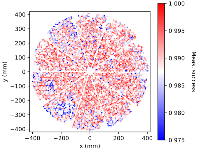
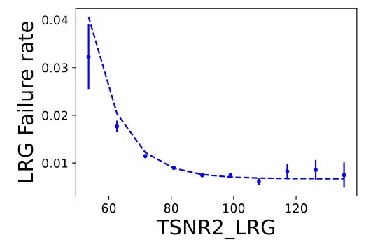
Redshift failures
Taken from Zhao et al. (2020)
- redshift efficiency involves the response of the telescope,
spectrograph and redshift determination pipeline - may vary with spectroscopic observing conditions / instrument
- corrected by a weight
Taken from Krolewski et al. 2024
Spectroscopic surveys: take-aways
Taken from Zhao et al. (2020)
-
\(\bar{n}\) varies due to photometry and spectroscopy:
-
angular photometric systematics
-
fibre assignment
-
redshift failures
-
- Understanding \(\bar{n}\) is key to reliable clustering measurements
-
Effects of systematics tested on fast simulations: mocks
Taken from Zhao et al. (2020)
Outline
- Past and current surveys
- Clustering observables
- Spectroscopic surveys and systematics
- Large-scale structure formation
- BAO and RSD theory models
- Current constraints
- Other clustering analyses
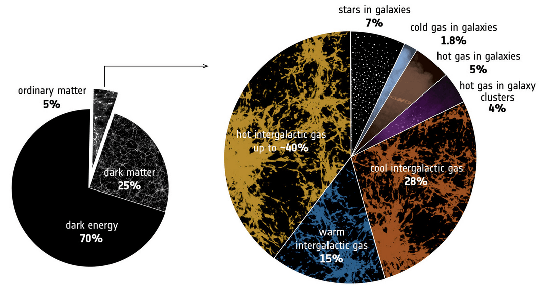
Galaxy - matter relation
How do galaxies "populate" the (dark) matter density field?
\Omega_\mathrm{cdm}
\Omega_\mathrm{b}
credit: ESA
galaxies:
14% of \(\Omega_\mathrm{b}\)
3% of \(\Omega_\mathrm{m}\)
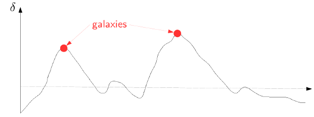
Galaxy bias
- galaxy formation in two steps (White and Rees 1978):
- dark matter forms halos = gravitationally-bound structures
- gas cools down, baryons aggregate into galaxies
- galaxies trace the density field, in large overdensities → bias
Galaxy bias
- galaxy formation in two steps (White and Rees 1978):
- dark matter forms halos = gravitationally-bound structures
- gas cools down, baryons aggregate into galaxies
- galaxies trace the density field, in large overdensities → bias
- on large scales
- halo model (e.g. Seljak 2000):
- galaxies ⇔ DM halos with halo occupation distribution
- DM halos ⇔ DM field with halo bias (Press and Schechter 1974, Bardeen et al. 1986, Sheth and Tormen 1999)
\delta_\mathrm{g} = \orange{b_1} \delta + \epsilon \Rightarrow P_\mathrm{gg}(k) = \orange{b_1}^2 P_\mathrm{\delta\delta}(k) + N_\epsilon
linear bias parameter
Poisson noise
Galaxy bias
- galaxy formation in two steps (White and Rees 1978):
- dark matter forms halos = gravitationally-bound structures
- gas cools down, baryons aggregate into galaxies
- galaxies trace the density field, in large overdensities → bias
- bias expansion (e.g. McDonald and Roy 2009):
\delta_\mathrm{g} = \orange{b_1} \delta + \orange{b_2} \delta^2 + \orange{b_s} s^2 + \orange{b_\nabla} \nabla \delta + \cdots
second order bias
shear bias
shear bias
non-local bias
shear bias
s^2 = s_{ij} s_{ji} \text{ with } s_{ij} = \left[\nabla_i \nabla_j \nabla^{-2} - \delta_{ij}^K / 3\right] \delta
Structure formation
- matter is described as a collisionless fluid that evolves only through gravitation, in an expanding Universe
- Gravity:
- First two moments of the Vlasov-Poisson equation:
\frac{\partial f}{\partial \eta}
+ \frac{\mathbf{p}}{ma} \cdot \frac{\partial f}{\partial \mathbf{x}}
- am \nabla \Phi \cdot \frac{\partial f}{\partial \mathbf{p}} = 0
\Delta \Phi = a^{2} 4\pi G_{N} \bar{\rho} \, \delta
= \frac{3}{2} a^2 H^{2} \Omega_\mathrm{m} \, \delta
\delta^\prime + \nabla_i \left[(1 + \delta) u_i \right] = 0
continuity equation
Euler equation
u_i^\prime + a H u_i + u_j \nabla_j u_i = - \nabla_i \Phi - \frac{1}{\rho} \nabla_j (\rho \sigma_{ij})
anisotropic stress tensor, sourced by multi-streams / shell-crossing
conformal time derivative \(d\eta = dt / a\)
velocity
Poisson equation
gravitational potential
Perturbation theory: first order
- Linear order Eulerian PT
- First order Lagrangian PT = Zeldovich approximation
\frac{\partial f}{\partial \eta}
+ \frac{\mathbf{p}}{ma} \cdot \frac{\partial f}{\partial \mathbf{x}}
- am \nabla \Phi \cdot \frac{\partial f}{\partial \mathbf{p}} = 0
\delta^{\prime\prime} + a H \delta^\prime - \frac{3}{2} \Omega_\mathrm{m} \delta = 0
\orange{D_{+}(a) = a}
linear growth factor
\theta = \nabla_i u_i = \orange{f} a H \delta
velocity divergence
\orange{f = \frac{d \ln D}{d \ln a}} \simeq \Omega_\mathrm{m}^{0.55}
logarithmic growth rate
\mathbf{x}(\eta) = \mathbf{q} + \mathbf{\Psi}(\mathbf{q}, \eta)
\mathbf{\Psi}(\mathbf{k}, \eta) = -\frac{i \mathbf{k}}{k^2} D_+(\eta) \delta_0(\mathbf{k})
\delta = D_{+} \delta_0
decreasing mode, and growing mode
Zeldovich displacement
Lagrangian picture
Perturbation theory: first order
- Linear order Eulerian PT
- First order Lagrangian PT = Zeldovich approximation
\frac{\partial f}{\partial \eta}
+ \frac{\mathbf{p}}{ma} \cdot \frac{\partial f}{\partial \mathbf{x}}
- am \nabla \Phi \cdot \frac{\partial f}{\partial \mathbf{p}} = 0
\delta^{\prime\prime} + a H \delta^\prime - \frac{3}{2} \Omega_\mathrm{m} \delta = 0
\orange{D_{+}(a) = a}
linear growth factor
\theta = \nabla_i u_i = \orange{f} a H \delta
velocity divergence
\orange{f = \frac{d \ln D}{d \ln a}} \simeq \Omega_\mathrm{m}^{0.55}
logarithmic growth rate
\mathbf{x}(\eta) = \mathbf{q} + \mathbf{\Psi}(\mathbf{q}, \eta)
\mathbf{\Psi}(\mathbf{k}, \eta) = \frac{i \mathbf{k}}{k^2} D_+(\eta) \delta_0(\mathbf{k})
\delta = D_{+} \delta_0
decreasing mode, and growing mode
Zeldovich displacement
Lagrangian picture
initial positions
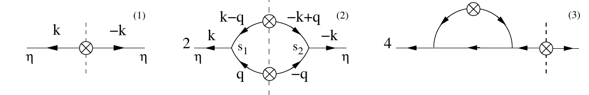
Perturbation theory: higher order
- Write \(\delta\) and \(\theta\) as an expansion:
\frac{\partial f}{\partial \eta}
+ \frac{\mathbf{p}}{ma} \cdot \frac{\partial f}{\partial \mathbf{x}}
- am \nabla \Phi \cdot \frac{\partial f}{\partial \mathbf{p}} = 0
\delta(\mathbf{k}) = D_+ \delta^{(1)}(\mathbf{k}) + \cdots + D_+^n \delta^{(n)}(\mathbf{k}) + \cdots
\delta^{(n)}(\mathbf{k}) = \int \frac{d^3 q_1 \cdots d^3 q_n}{(2\pi)^{3(n - 1)}} \delta_D(\mathbf{k} - \mathbf{q}_1 - \cdots - \mathbf{q}_n) \orange{F^{(n)}(\mathbf{q}_1, \cdots, \mathbf{q}_n)} \delta_0(\mathbf{q}_1) \cdots \delta_0(\mathbf{q}_n)
perturbation theory kernels
(geometrical functions of \(\mathbf{q}\)'s that can be computed recursively)
- Diagrammatic representation, up to order 3:
2
\(\mathbf{q}_1\)
\(\mathbf{q}_2\)
\(\mathbf{q}_1\)
\(\mathbf{q}_2\)
\(\mathbf{q}_3\)
\(\mathbf{k}\)
\(\mathbf{k}\)
\(\mathbf{k}\)
+
+
- Using Wick's theorem, compute any \(n\)-point statistics, e.g. \(P_{\delta\delta}(\mathbf{k})\) at 1-loop
Taken from Crocce & Scoccimarro
\langle \delta_{a_1}(\mathbf{k}_1) \cdots \delta_{a_{2n}}(\mathbf{k}_{2n}) \rangle
= \sum_{\text{all pair associations}}
\prod_{\text{pairs } (i,j) \in p}
\langle \delta_{a_i}(\mathbf{k}_i)\, \delta_{a_j}(\mathbf{k}_j) \rangle
Taken from Zhao et al. (2020)
N-body simulations
solve numerically the Vlasov-Poisson equations for the dark matter fluid by sampling the phase-space with particles
N-body simulations
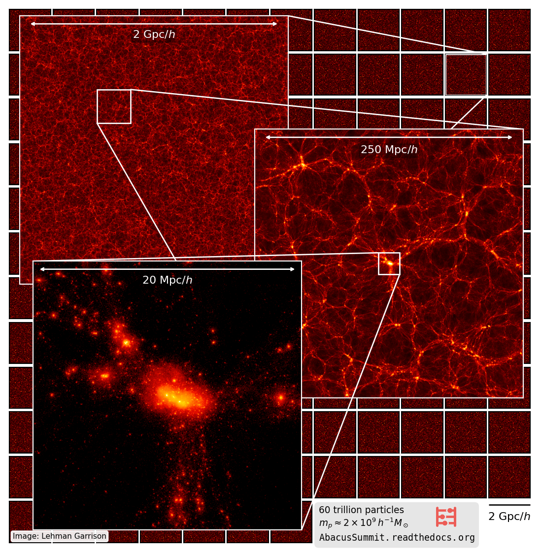
Credit: The AbacusSummit Team
- Dark matter particles virialize into dark matter halos
- Halo finders (Friend-of-Friend, Spherical Overdensity, Rockstar...)
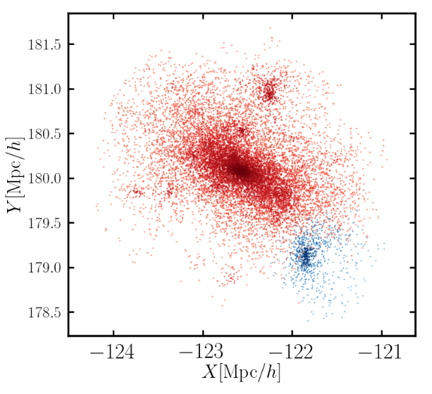
Adapted from Hadzhiyska et al. 2021
Taken from Zhao et al. (2020)
Halo occupation distribution
specify the probability to find \(N\) galaxies in a halo of mass \(M\)
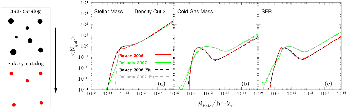
Right: HOD measured on the outputs of two semi-analytical models (GALFORM and LGALAXIES) run on the Millennium simulation. Taken from Contreras et al. (2013).
- split between central and satellite galaxies
- also sample galaxy velocities
- many extensions (assembly bias = dependence on other properties (e.g. local density or shear)
Taken from Zhao et al. (2020)
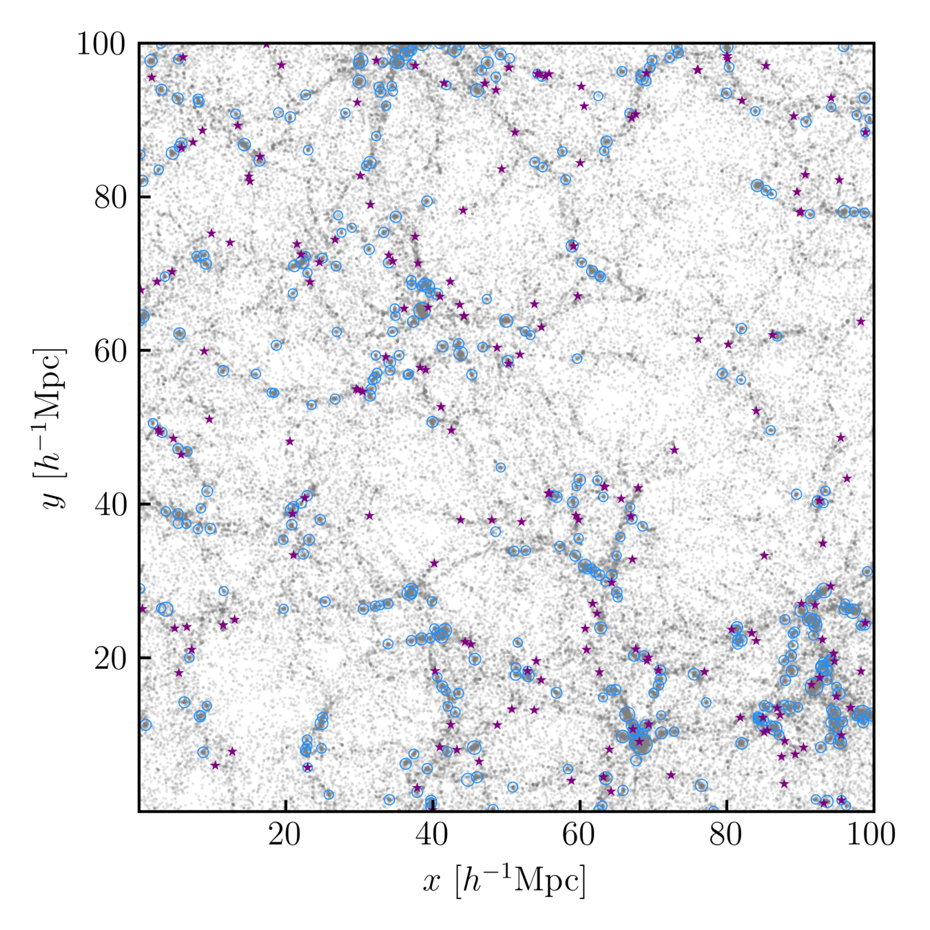
halos
emission line galaxies
Credit: Mathilde Pinon
Halo occupation distribution
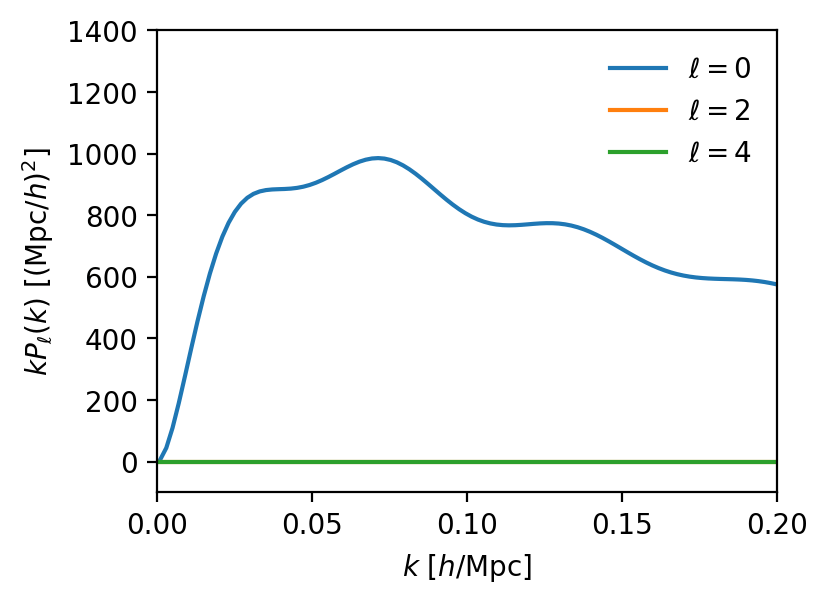
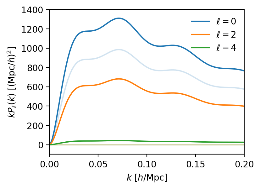
LSS formation: take-aways
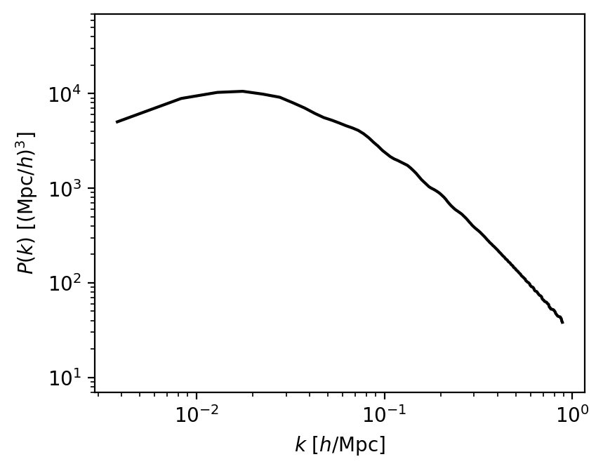
linear matter power spectrum
LSS formation: take-aways
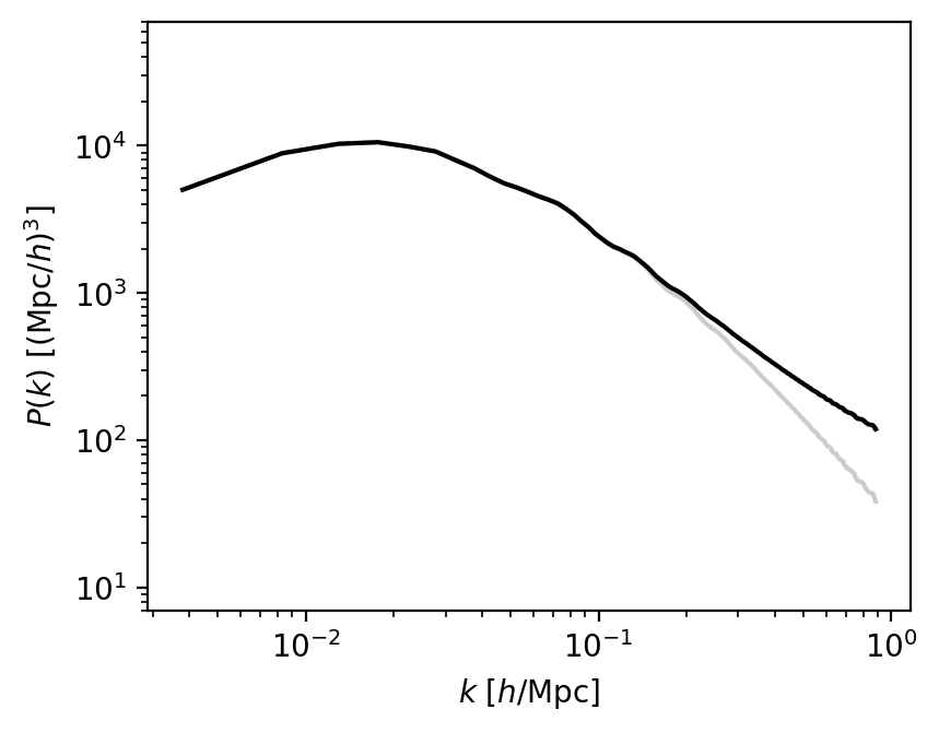
evolved matter power spectrum (\(z = 0.8\))
LSS formation: take-aways
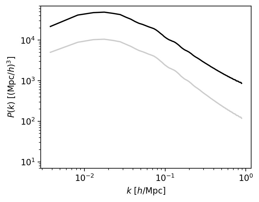
galaxy power spectrum (\(z = 0.8\))
Interlude: the primordial power spectrum
- The initial power spectrum (of density fluctuations after the inflaction) is:
P_{\delta\delta}^\mathrm{ini}(k) \propto \orange{A_s} \left(\frac{k}{k_\mathrm{pivot}}\right)^{\orange{n_\mathrm{s}}}
scalar index
amplitude
- Early Universe is dominated by radiation:
- \(k \ll H a \equiv \mathcal{H}\), \(\delta\) grows as \(a\) (scale factor)
- \(k \gg \mathcal{H}\) (Jeans scale), growth suppressed by radiation pressure: \(\delta\) constant or logarithmically growing
- At \(z_\mathrm{eq}\), matter - radiation equality: \(\delta\) grows as \(a\)
\(\Rightarrow\) characteristic "equality" scale \(k_\mathrm{eq} = \mathcal{H}_\mathrm{eq}\)
- Encoded in the transfer function
P_{\delta\delta}(k) = \orange{T(k)}^2 P_{\delta\delta}^\mathrm{ini}(k)
\orange{T(k) \propto \left\lbrace
\begin{align*}
1 & \qquad k \ll k_\mathrm{eq}\\
(k_\mathrm{eq} / k)^2 & \qquad k \gg k_\mathrm{eq}
\end{align*}
\right.}
Interlude: the primordial power spectrum
- The initial power spectrum (of density fluctuations after the inflaction) is:
P_{\delta\delta}^\mathrm{ini}(k) \propto \orange{A_s} \left(\frac{k}{k_\mathrm{pivot}}\right)^{\orange{n_\mathrm{s}}}
scalar index
amplitude
P_{\delta\delta}(k) = \orange{T(k)}^2 P_{\delta\delta}^\mathrm{ini}(k)
- Early Universe is dominated by radiation:
- \(k \ll H a \equiv \mathcal{H}\), \(\delta\) grows as \( \mathcal{H}^{-2} \)
- \(k \gg \mathcal{H}\) (Jeans scale), growth suppressed by radiation pressure: \(\delta\) constant or logarithmically growing
- After \(z_\mathrm{eq}\), matter - radiation equality: \(\delta\) grows as \( a \propto \mathcal{H}^{-2} \)
\(\Rightarrow\) characteristic "equality" scale \(k_\mathrm{eq} = \mathcal{H}_\mathrm{eq}\)
- Encoded in the transfer function
Interlude: the primordial power spectrum
- The initial power spectrum (of density fluctuations after the inflaction) is:
P_{\delta\delta}^\mathrm{ini}(k) \propto \orange{A_s} \left(\frac{k}{k_\mathrm{pivot}}\right)^{\orange{n_\mathrm{s}}}
scalar index
amplitude
- Early Universe is dominated by radiation:
- \(k \ll H a \equiv \mathcal{H}\), \(\delta\) grows as \( \mathcal{H}^{-2} \)
- \(k \gg \mathcal{H}\) (Jeans scale), growth suppressed by radiation pressure: \(\delta\) constant or logarithmically growing
- After \(z_\mathrm{eq}\), matter - radiation equality: \(\delta\) grows as \( a \propto \mathcal{H}^{-2} \)
\(\Rightarrow\) characteristic "equality" scale \(k_\mathrm{eq} = \mathcal{H}_\mathrm{eq}\)
- Encoded in the transfer function
P_{\delta\delta}(k) = \orange{T(k)}^2 P_{\delta\delta}^\mathrm{ini}(k)
\orange{T(k) \propto \left\lbrace
\begin{align*}
1 & \qquad k \ll k_\mathrm{eq}\\
(k_\mathrm{eq} / k)^2 & \qquad k \gg k_\mathrm{eq}
\end{align*}
\right.}
Interlude: the primordial power spectrum
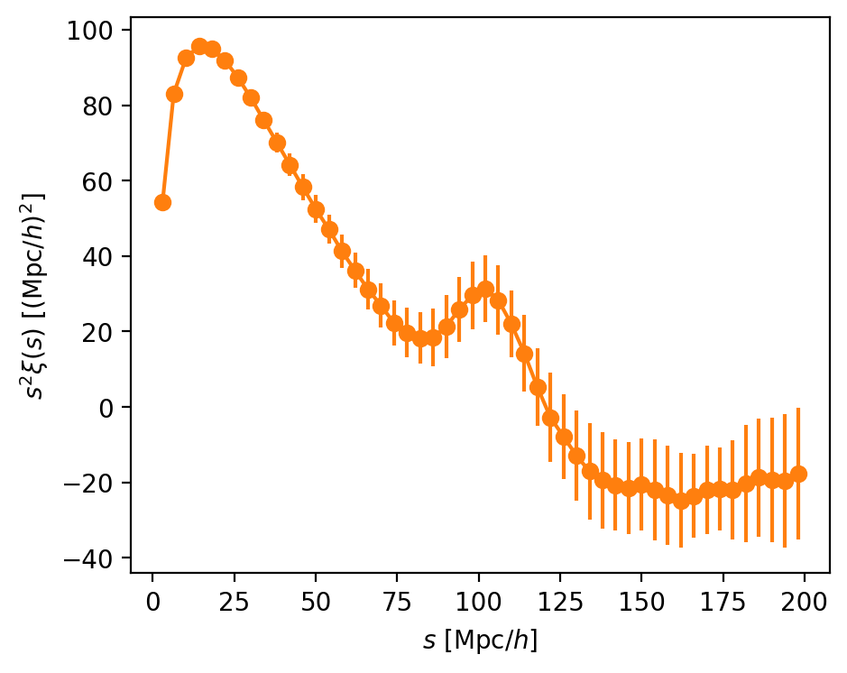
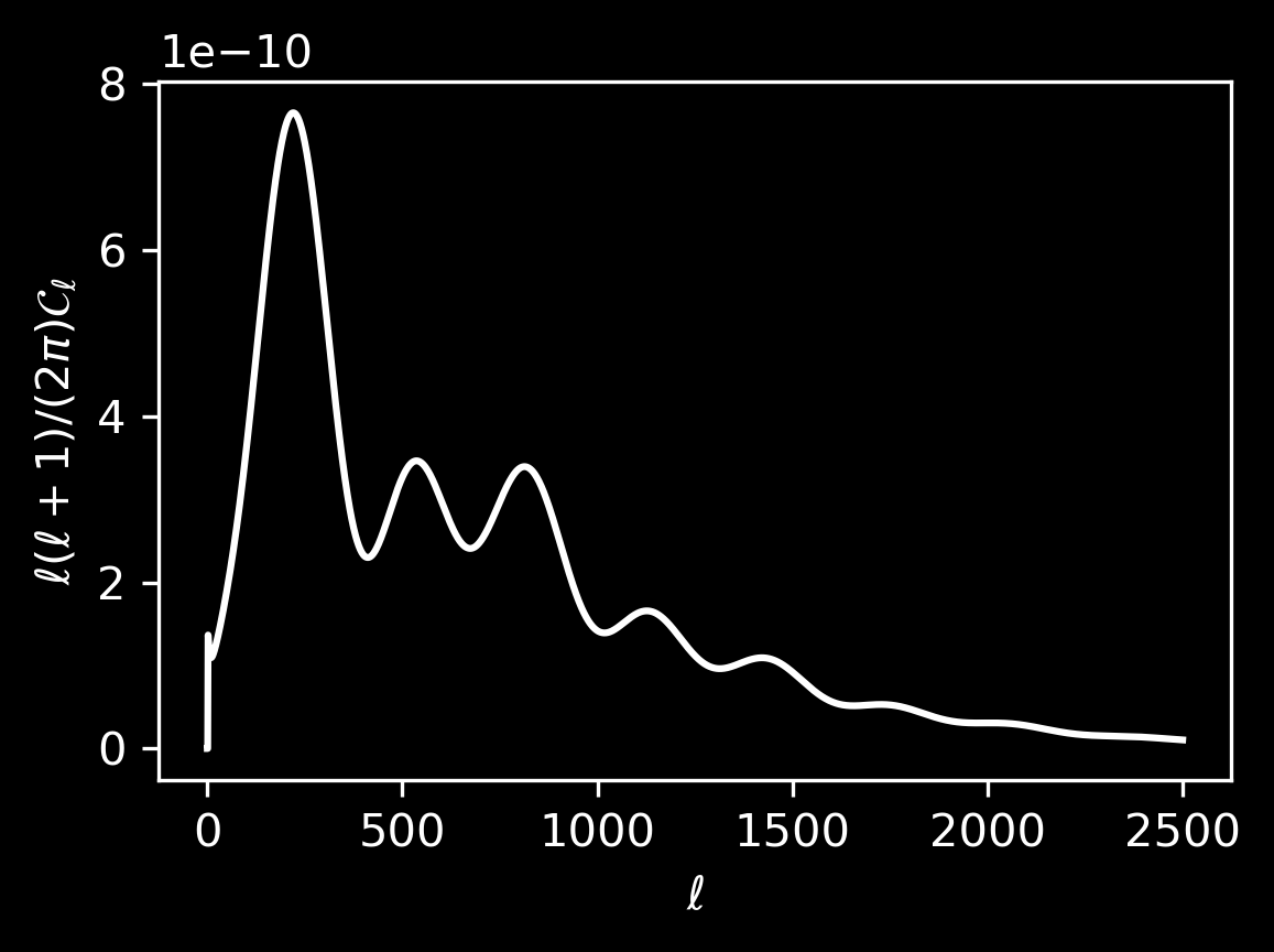
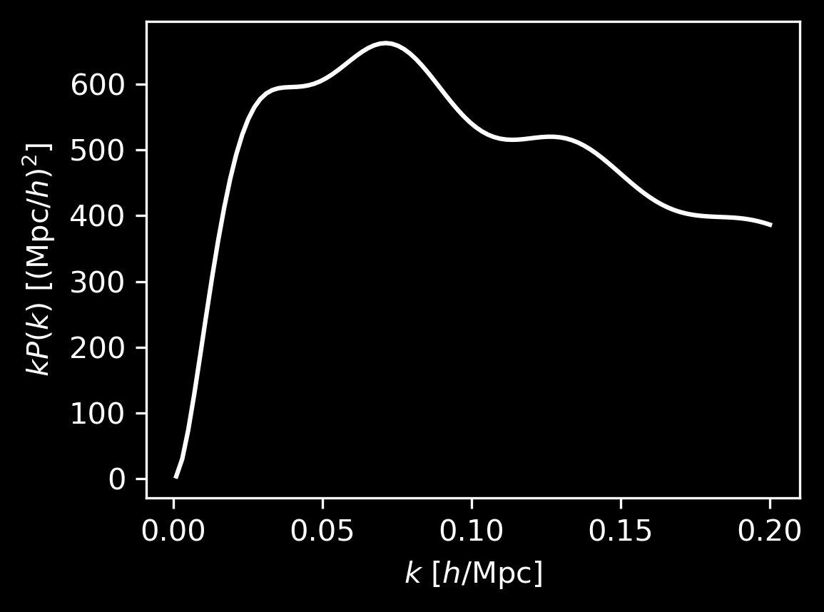
Features
peak
oscillations
What are the noticeable features in \(\xi_\mathrm{gg}(s)\) or \(P_\mathrm{gg}(k)\)?
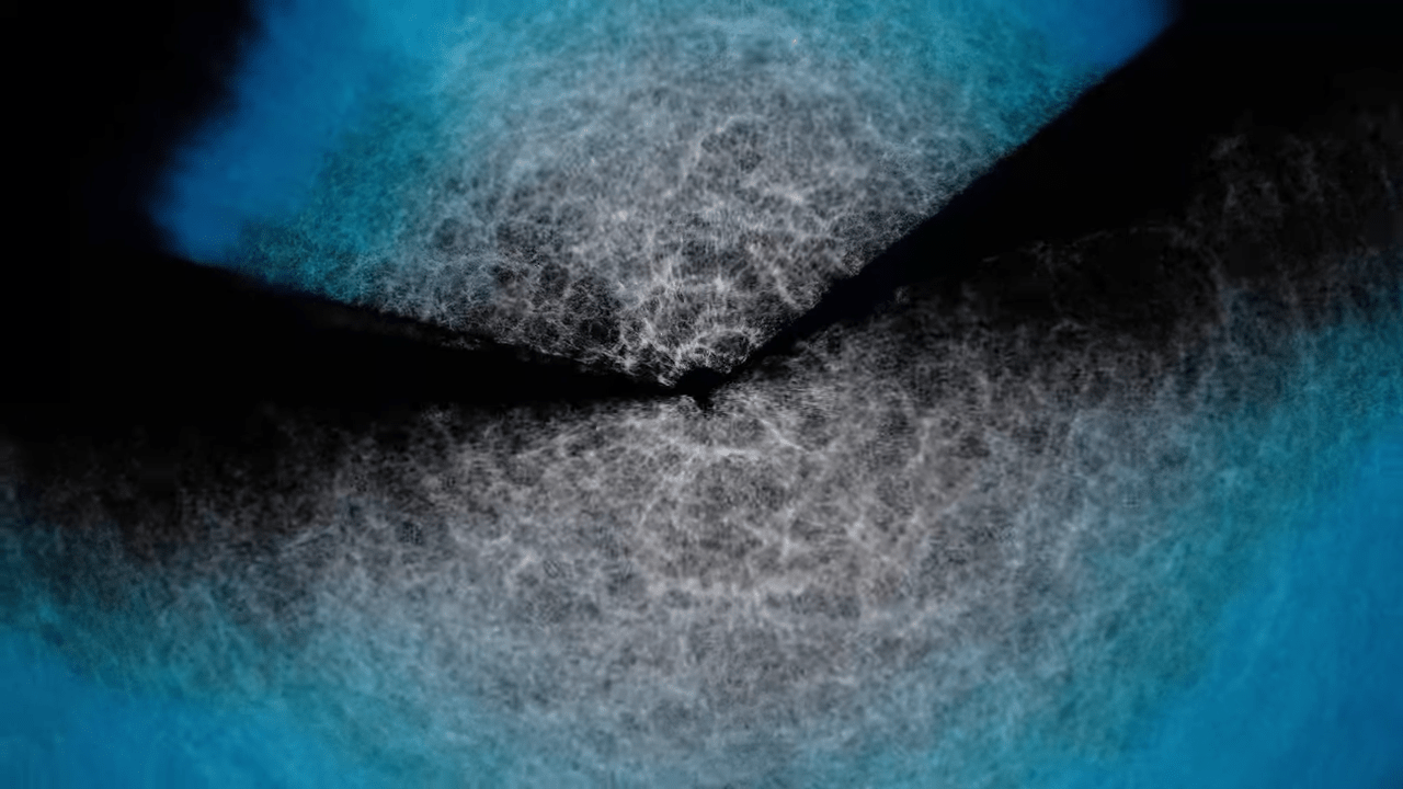
Baryon acoustic oscillations (BAO)
Sound waves in primordial plasma
At recombination (\(z \simeq 1100\))
- plasma changes to optically thin
- baryons decouple from photons
- sound wave stalls after travelling \(r_\mathrm{d}\)
Sound horizon scale at the drag epoch
\(r_\mathrm{d} \simeq 150\; \mathrm{Mpc}\)
Baryon acoustic oscillations (BAO)
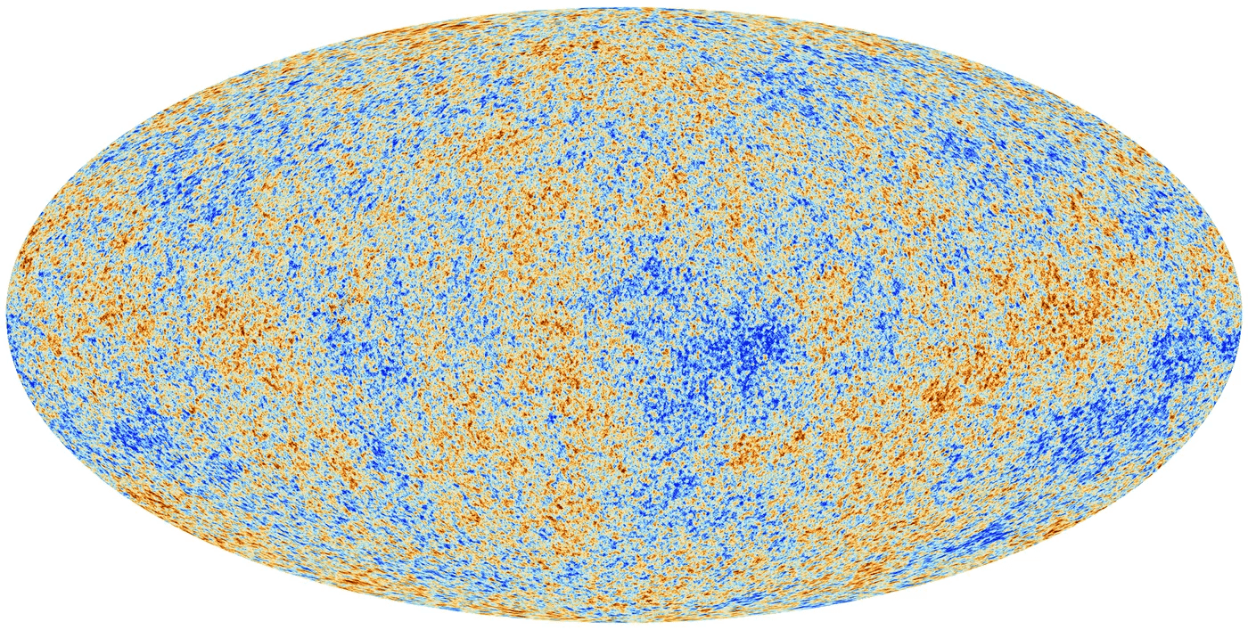
CMB (\(z \simeq 1100\))
At recombination (\(z \simeq 1100\))
- plasma changes to optically thin
- baryons decouple from photons
- sound wave stalls after travelling \(r_\mathrm{d}\)
Sound horizon scale at the drag epoch
\(r_\mathrm{d} \simeq 150\; \mathrm{Mpc}\)
Sound waves in primordial plasma
Baryon acoustic oscillations (BAO)
CMB (\(z \simeq 1100\))
Baryon acoustic oscillations (BAO)
Thanks to Julian Bautista!
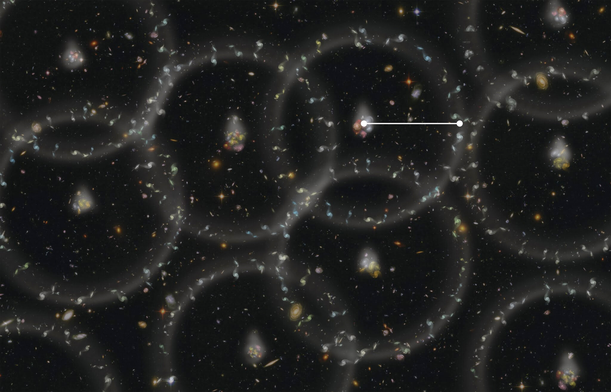
BAO
Credits: CAASTRO, https://www.youtube.com/watch?v=jpXuYc-wzk4
Baryon acoustic oscillations (BAO)
distribution of galaxies (cartoonish)
\theta_\mathrm{BAO} = r_\mathrm{d} / D_\mathrm{M}(z)
transverse comoving distance
sound horizon \(r_\mathrm{d}\)
Let's measure:
- angle on the sky (transverse to the line-of-sight): \(\theta_\mathrm{BAO} = \orange{r_\mathrm{d}}/\green{D_\mathrm{M}(z)}\)
- \(\Delta z\) (along the line-of-sight): \( \Delta z_\mathrm{BAO} = r_\mathrm{d} / D_\mathrm{H}(z) = \green{H(z)} \orange{r_\mathrm{d}} / c \)
Baryon acoustic oscillations (BAO)
Let's measure:
- angle on the sky (transverse to the line-of-sight): \(\theta_\mathrm{BAO} = \orange{r_\mathrm{d}}/\green{D_\mathrm{M}(z)}\)
- \(\Delta z\) (along the line-of-sight): \( \Delta z_\mathrm{BAO} = \orange{r_\mathrm{d}} / \green{D_\mathrm{H}(z)} = \green{H(z)} \orange{r_\mathrm{d}} / c \)
distribution of galaxies (cartoonish)
\Delta z_\mathrm{BAO} = r_\mathrm{d} / D_\mathrm{H}(z)
Hubble distance \(c/H(z)\)
sound horizon \(r_\mathrm{d}\)
Baryon acoustic oscillations (BAO)
Let's measure:
- angle on the sky (transverse to the line-of-sight): \(\theta_\mathrm{BAO} = \orange{r_\mathrm{d}}/\green{D_\mathrm{M}(z)}\)
- \(\Delta z\) (along the line-of-sight): \( \Delta z_\mathrm{BAO} = \orange{r_\mathrm{d}} / \green{D_\mathrm{H}(z)} = \green{H(z)} \orange{r_\mathrm{d}} / c \)
- at multiple redshifts \(z\)
Probes the expansion history (\(\green{D_\mathrm{M}, D_H}\)), hence the energy content (e.g. dark energy)
Absolute size at \(z = 0\): \(H_0 \orange{r_\mathrm{d}}\)
z_1
z_2
z_3
Baryon acoustic oscillations (BAO)
correlation function
\alpha_\mathrm{iso} \propto (D_{\mathrm{M}}^{2}(z) D_\mathrm{H}(z))^{1/3} / r_\mathrm{d}
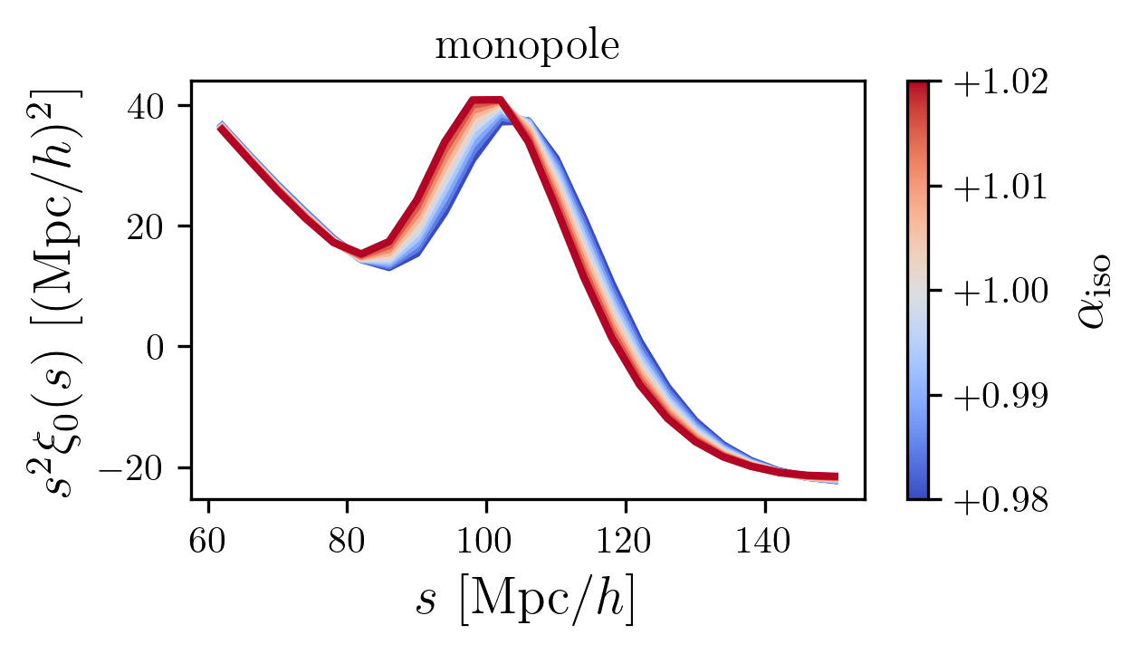
BAO peak
line-of-sight
monopole
isotropic
comoving transverse distance
Hubble distance \(c/H(z)\)
sound horizon (standard ruler)
Baryon acoustic oscillations (BAO)
isotropic
anisotropic
\propto D_{\mathrm{M}}(z) / D_\mathrm{H}(z)
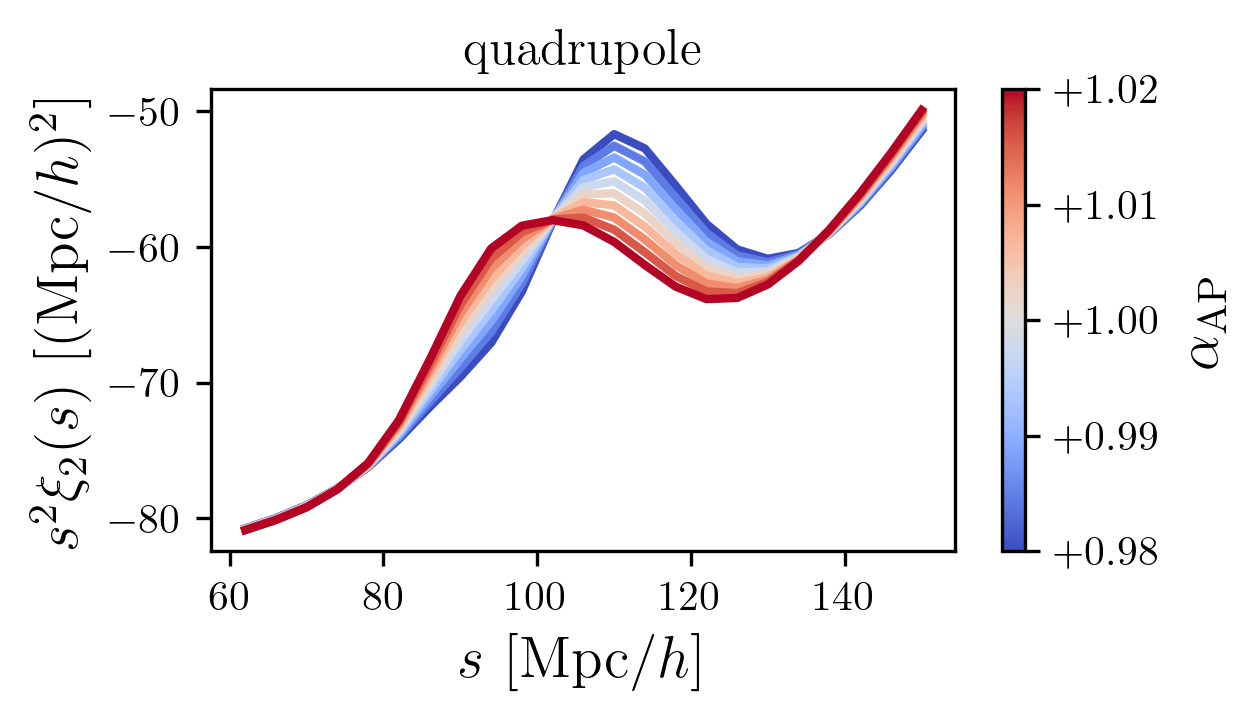
BAO peak
line-of-sight
monopole
quadrupole
\propto (D_{\mathrm{M}}^{2}(z) D_\mathrm{H}(z))^{1/3} / r_\mathrm{d}
line-of-sight
Q: What can make the BAO look anisotropic?
Alcock-Paczynski effect
R.A., Dec., \(z\) \(\Rightarrow\) \(\mathbf{x}\) with the true cosmology
Alcock-Paczynski effect
\(\propto q_\parallel = D_\mathrm{H}^\mathrm{fid}(z) / D_\mathrm{H}(z) \)
R.A., Dec., \(z\) \(\Rightarrow\) \(\mathbf{x}\) with wrong (fiducial) cosmology
\(\propto q_\perp = D_\mathrm{M}^\mathrm{fid}(z) / D_\mathrm{M}(z) \)
Alcock-Paczynski effect
In the theory:
\left\lbrace \begin{align*}
&q_\parallel = D_\mathrm{H}(z) / D_\mathrm{H}^\mathrm{fid}(z)\\
&q_\perp = D_\mathrm{M}(z) / D_\mathrm{M}^\mathrm{fid}(z)
\end{align*} \right .
P^\mathrm{fid}(k_\parallel, k_\perp) = 1 / (\orange{q_\parallel q_\perp}^2) P(k_\parallel / \orange{q_\parallel}, k_\perp / \orange{q_\perp})
\Rightarrow P^\mathrm{fid}(k, \mu) = 1 / (\orange{q_\parallel q_\perp}^2) P(k^\prime, \mu^\prime)
rescaled in fiducial coordinates
\left\lbrace \begin{align*}
k^\prime &= \frac{k}{\orange{q_\perp}} \left[ 1 + \mu^2 \left( \frac{\orange{q_\perp}^2}{\orange{q_\parallel}^2} - 1 \right) \right]^{1/2}\\
\mu^\prime &= \frac{\mu \orange{q_\perp}}{\orange{q_\parallel}} \left[ 1 + \mu^2 \left( \frac{\orange{q_\perp}^2}{\orange{q_\parallel}^2} - 1 \right) \right]^{-1/2}
\end{align*}\right .
\(\propto q_\parallel\)
\(\propto q_\perp \)
Features
non-zero quadrupole!
What are the noticeable features in \(\xi_\mathrm{gg}(s)\) or \(P_\mathrm{gg}(k)\)?
non-zero quadrupole!
Q: where do you think it (mainly) comes from?
Redshift space distortions (RSD)
observed redshifts (\(z_\mathrm{obs}\)) =
Hubble flow (\(\blue{z_\mathrm{cosmo}}\))
+ peculiar velocities (\(\orange{u_z/c}\))
+ (relativistic terms)
redshift-space positions (\(\mathbf{s}\)) =
real space position (\(\blue{\mathbf{r}}\))
+ RSD shift (\(\orange{u_z/H\mathbf{\hat{z}}}\))
u_z \propto f\sigma_8
Redshift space distortions (RSD)
observed redshifts (\(z_\mathrm{obs}\)) =
Hubble flow (\(\blue{z_\mathrm{cosmo}}\))
+ peculiar velocities (\(\orange{u_z/c}\))
+ (relativistic terms)
redshift-space positions (\(\mathbf{s}\)) =
real space position (\(\blue{\mathbf{r}}\))
+ RSD shift (\(\orange{u_z/H\mathbf{\hat{z}}}\))
\(s = D_\mathrm{c}(z_\mathrm{obs})\)
u_z \propto f\sigma_8
Redshift space distortions (RSD)
real-space
Credit: Mathilde Pinon
Redshift space distortions (RSD)
redshift-space
Credit: Mathilde Pinon
Redshift space distortions (RSD)
galaxy positions in redshift space: \(\mathbf{s} = \mathbf{r} - v_z \hat{z}\) with \(v_z = -\frac{\mathbf{u} \cdot \hat{z}}{H}\)
mass conservation:
\([1 + \delta_s(\mathbf{s})] d^3s = [1 + \delta_r(\mathbf{r})] d^3r \implies \delta_s(\mathbf{s}) = \left[ 1 + \delta_r(\mathbf{r}) \right] \left| \frac{d^3 s}{d^3 r} \right|^{-1} - 1 \)
power spectrum in redshift space:
P_s(\mathbf{k}) = \int d^3x e^{i \mathbf{k} \cdot \mathbf{x}} \left\langle \textcolor{red}{e^{-i k_\mu \Delta v_z}} \textcolor{blue}{\left[ \delta_r(\mathbf{r}) + \partial_z v_z(\mathbf{r}) \right] \left[ \delta_r(\mathbf{r} + \mathbf{x}) + \partial_z v_z(\mathbf{r} + \mathbf{x}) \right]} \right\rangle
Kaiser: \(\delta_r + \partial_z v_z \rightarrow (b_1 + f \mu^2)\delta\) in linear theory, enhancement on large scales
Finger-of-God: \(e^{-ik_\mu \Delta v_z}\) damping on scales \(\lesssim 3\, \mathrm{Mpc}\)
Kaiser
Redshift space distortions (RSD)
galaxy positions in redshift space: \(\mathbf{s} = \mathbf{r} - v_z \hat{z}\) with \(v_z = -\frac{\mathbf{u} \cdot \hat{z}}{H}\)
mass conservation:
\([1 + \delta_s(\mathbf{s})] d^3s = [1 + \delta_r(\mathbf{r})] d^3r \implies \delta_s(\mathbf{s}) = \left[ 1 + \delta_r(\mathbf{r}) \right] \left| \frac{d^3 s}{d^3 r} \right|^{-1} - 1 \)
power spectrum in redshift space:
P_s(\mathbf{k}) = \int d^3x e^{i \mathbf{k} \cdot \mathbf{x}} \left\langle \textcolor{red}{e^{-i k_\mu \Delta v_z}} \textcolor{blue}{\left[ \delta_r(\mathbf{r}) + \partial_z v_z(\mathbf{r}) \right] \left[ \delta_r(\mathbf{r} + \mathbf{x}) + \partial_z v_z(\mathbf{r} + \mathbf{x}) \right]} \right\rangle
Kaiser: \(\delta_r + \partial_z v_z \rightarrow (b_1 + f \mu^2)\delta\) in linear theory, enhancement on large scales
Finger-of-God: \(e^{-ik_\mu \Delta v_z}\) damping on scales \(\lesssim 3\, \mathrm{Mpc}\)
Finger-of-God
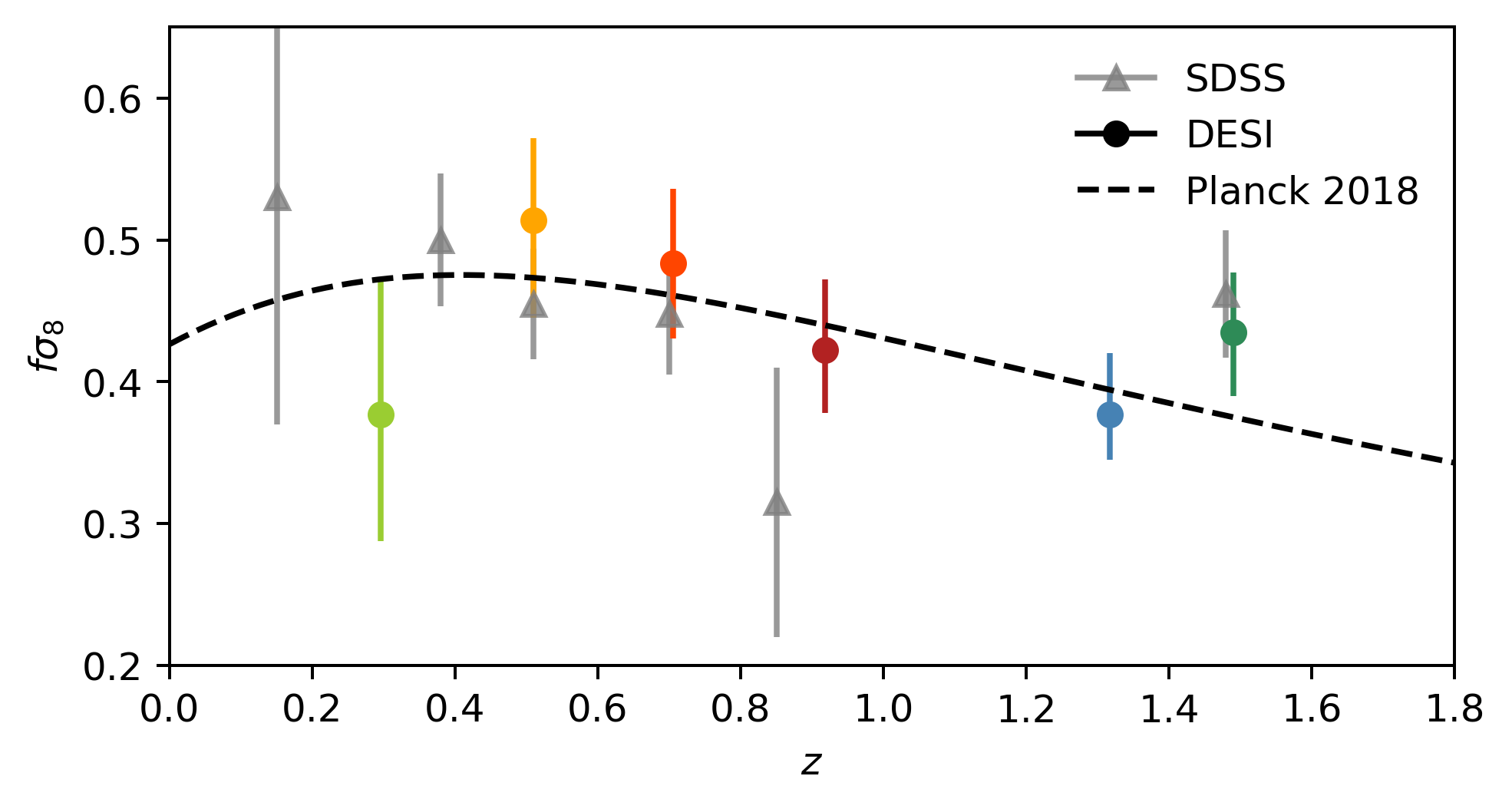
Measurement of \(f\sigma_8\)
\(P_s(k, \mu) = (b_1 + f \mu^2)^2 P_{\delta\delta}(k) = b_1^2 (1 + \beta \mu^2)^2 P_{\delta\delta}(k)\)
Kaiser model (= linear order)
with \(\beta = f / b_1\). Equivalently:
P_s(k, \mu) = \left(\beta^{-1} + \mu^2\right)^2 P_{\theta\theta}(k)
(for historical reasons) at a pivot point of \(8\;\mathrm{Mpc}/h\)
\(= f \sigma_8\) with \(f = \frac{d \ln D}{d \ln a} \simeq \Omega_\mathrm{m}^{0.55}\) within ΛCDM
probe matter density \(\Omega_\mathrm{m}\) / test of general relativity
Typically bias is marginalised over:
effectively measure the (amplitude of) the velocity divergence power spectrum \(P_{\theta\theta}(k)\)
BAO and RSD: take-aways
RSD
RSD
BAO
Anisotropic correlation function or power spectrum of galaxies. Sensitive to:
- RSD: \(f\sigma_8\) ⇒ energy content, test of general relativity
- BAO: \(D_M / r_\mathrm{d} , D_H /r_\mathrm{d}\) ⇒ energy content
- more generally: primordial power spectrum (inflation, matter-radiation equality), neutrinos, etc.
Taken from Zhao et al. (2020)
Outline
- Past and current surveys
- Clustering observables
- Spectroscopic surveys and systematics
- Large-scale structure formation
- BAO and RSD theory models
- Current constraints
- Other clustering analyses
Taken from Zhao et al. (2020)
BAO model
- measure only the position of the BAO peak: robust
- split fiducial power spectrum \(P(k)\) into no-wiggle \(P_\mathrm{nw}(k)\) and wiggles \(P_\mathrm{w}(k) = P(k) - P_\mathrm{nw}(k)\)
- marginalize over the shape: broadband parameters (polynomials)
- adjust position of wiggles \(P_\mathrm{w}(k^\prime)\)

P_\mathrm{gg}(k, \mu) = \green{\mathcal{B}(k, \mu) P_\mathrm{nw}(k)} + \mathcal{C}(k^\prime, \mu^\prime) \red{P_\mathrm{w}(k^\prime)} + \blue{\mathcal{D}(k, \mu)}
"no-wiggle Kaiser"
- correlation function = Hankel transform(power spectrum)
\left\lbrace \begin{align*}
k^\prime &= \frac{k \orange{\alpha_\mathrm{ap}}^{1/3}}{\orange{\alpha_\mathrm{iso}}} \left[ 1 + \mu^2 \left( \orange{\alpha_\mathrm{ap}}^{-2} - 1 \right) \right]^{1/2}\\
\mu^\prime &= \frac{\mu}{\orange{\alpha_\mathrm{ap}}} \left[ 1 + \mu^2 \left( \orange{\alpha_\mathrm{ap}}^{-2} - 1 \right) \right]^{-1/2}
\end{align*} \right.
Non-linear structure growth and peculiar velocities blur and shrink (slightly) the ruler

Eisenstein et al. 2008, Padmanabhan et al. 2012
BAO reconstruction
reconstruction
Estimates Zeldovich displacements from observed field and moves galaxies back: refurbishes the ruler (improves precision and accuracy)
reconstruction
BAO reconstruction
BAO reconstruction

Credit: DESI
Taken from Zhao et al. (2020)
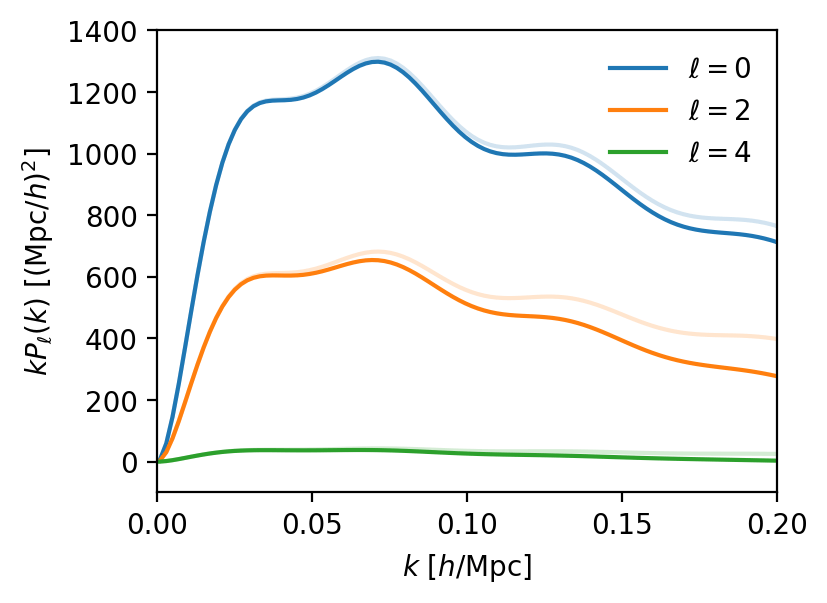
Full Shape models
Unbiased measurement of amplitude \(f\sigma_8\) ⇒ accurate model for the full shape power spectrum.
Various approaches (% accuracy at \(z = 1\)):
- WiggleZ (Blake, 2010): Halofit \(P_\mathrm{m}(k)\) + Kaiser + FoG
- in BOSS/eBOSS (< 2020): perturbation theory models:
- power spectrum: standard/regularized PT (RPT, RegPT Taruya et al. 2012), RSD (Taruya et al. 2010), bias expansion (McDonald and Roy 2009) (\(k < 0.2 \; h/\mathrm{Mpc}\))
- correlation function: Gaussian streaming model (Reid and White 2011) (\(s > 30 \; \mathrm{Mpc}/h\))
Taken from Zhao et al. (2020)
Full Shape models
Unbiased measurement of amplitude \(f\sigma_8\) ⇒ accurate model for the full shape power spectrum.
Various approaches (% accuracy at \(z = 1\)):
- WiggleZ (Blake, 2010): Halofit \(P_\mathrm{m}(k)\) + Kaiser + FoG
- in BOSS/eBOSS (< 2020): perturbation theory models:
- power spectrum: standard/regularized PT (RPT, RegPT Taruya et al. 2012), RSD (Taruya et al. 2010), bias expansion (McDonald and Roy 2009) (\(k < 0.2 \; h/\mathrm{Mpc}\))
- correlation function: Gaussian streaming model (Reid and White 2011) (\(s > 30 \; \mathrm{Mpc}/h\))
- in DESI, Euclid, effective field theory: small-scale-sourced counterterm to regularize loop integrals (pybird, CLASS-PT, velocileptors, folps...) (\(k < 0.25 \; h/\mathrm{Mpc}\))
Taken from Zhao et al. (2020)
EFT models
P_{s, g}(k, \mu) = \blue{P^\mathrm{PT}(k, \mu)} + \orange{(b + f\mu^2) (b \alpha_0 + f\alpha_2 \mu^2 + f\alpha_4 \mu^4) k^2 P_{s, b_1^2}(k)} + \purple{\mathrm{SN}_0 + \mathrm{SN}_2 k^2 \mu^2 + \mathrm{SN}_4 k^4 \mu^4}
perturbation theory term = \(f(P_\mathrm{lin}, f)\)
linear and quasi-linear physics
counter-terms contribution
truncation of perturbative series
stochastic-terms contribution
small-scale galaxy physics
The Effective Field Theory in a nutshell
- perturbation theory model + counter-terms and stochastic terms
- dependence on cosmology into \(P_\mathrm{lin}(k)\), \(f\) and Alcock-Paczynski transform (\(\mathrm{R.A.}, \mathrm{Dec.}, z \Rightarrow \text{fiducial coordinates}\))
Taken from Zhao et al. (2020)
Full Shape models
Unbiased measurement of amplitude \(f\sigma_8\) ⇒ accurate model for the full shape power spectrum.
Various approaches (% accuracy at \(z = 1\)):
- WiggleZ (Blake, 2010): Halofit \(P_\mathrm{m}(k)\) + Kaiser + FoG
-
in BOSS/eBOSS (< 2020): perturbation theory models:
- power spectrum: standard/regularized PT (RPT, RegPT Taruya et al. 2012), RSD (Taruya et al. 2010), bias expansion (McDonald and Roy 2009) (\(k < 0.2 \; h/\mathrm{Mpc}\))
- correlation function: Gaussian streaming model (Reid and White 2011) (\(s > 30 \; \mathrm{Mpc}/h\))
- in DESI, Euclid, effective field theory: small-scale-sourced counterterm to regularize loop integrals (pybird, CLASS-PT, velocileptors, folps...) (\(k < 0.25 \; h/\mathrm{Mpc}\))
- hybrid PT/HOD models, e.g. Hand et al. 2017 (\(k < 0.4 \; h/\mathrm{Mpc}\))
- simulation-based models, e.g. SimBig Lemos et al. 2023
Taken from Zhao et al. (2020)
Mock challenge
Test the theoretical model accuracy against simulations (mocks)
Mock challenge
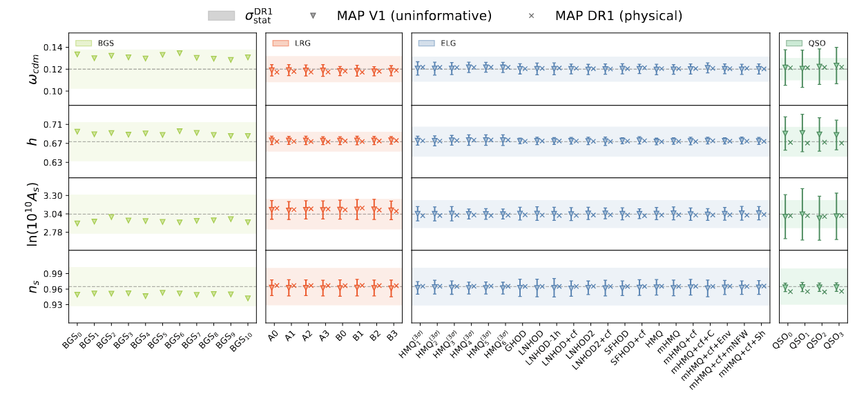
Taken from Findlay et al. 2024
fitted cosmological parameters
HOD-variations for each tracer (conformity, assembly bias, etc.)
Theory models: take-aways
Taken from Zhao et al. (2020)
- BAO models: fit the position of the BAO feature, marginalize over the shape of the power spectrum ("broadband")
- Full Shape models: full shape of the power spectrum, linear and quasi-linear scales. State-of-the-art of standard analyses: EFT models
- tested with N-body mock challenge
Likelihood
Taken from Zhao et al. (2020)
We usually assume a Gaussian likelihood
\ln{p(\mathbf{d} | \mathbf{\theta})} \propto -\frac{1}{2} (\mathbf{d} - \orange{\mathbf{t}}(\red{\mathbf{\theta}}))^T \green{\mathrm{C}}^{-1} (\mathbf{d} - \orange{\mathbf{t}}(\red{\mathbf{\theta}}))
theory model
data vector
(\(P_\ell(k)\) or \(\xi_\ell(s)\))
parameters
covariance matrix
- Full Shape fit: \(A_\mathrm{s} \text{ or }\sigma_8, \omega_\mathrm{cdm}, h, n_\mathrm{s}\)
- BAO fit: \(\alpha_\mathrm{iso}, \alpha_\mathrm{ap}\)
+ bias or "nuisance" parameters
analytic or based on fast simulations
We sample the posterior \(p(\red{\mathbf{\theta}} | \mathbf{d}) \propto p(\mathbf{d} | \red{\mathbf{\theta}}) \red{p(\mathbf{\theta})}\)
prior
In a nutshell
Taken from Zhao et al. (2020)

galaxy catalog
galaxy power spectrum (or correlation function)
cosmological constraints
compression = "we measure specific features"
e.g. BAO model \(\Rightarrow\) \(\alpha_\mathrm{iso}, \alpha_\mathrm{ap}\)

"variance of the density field as a function of scale"
Full Shape
Taken from Zhao et al. (2020)
Outline
- Past and current surveys
- Clustering observables
- Spectroscopic surveys and systematics
- Large-scale structure formation
- BAO and RSD theory models
- Current constraints
- Other clustering analyses
Taken from Zhao et al. (2020)
DESI DR1 BAO
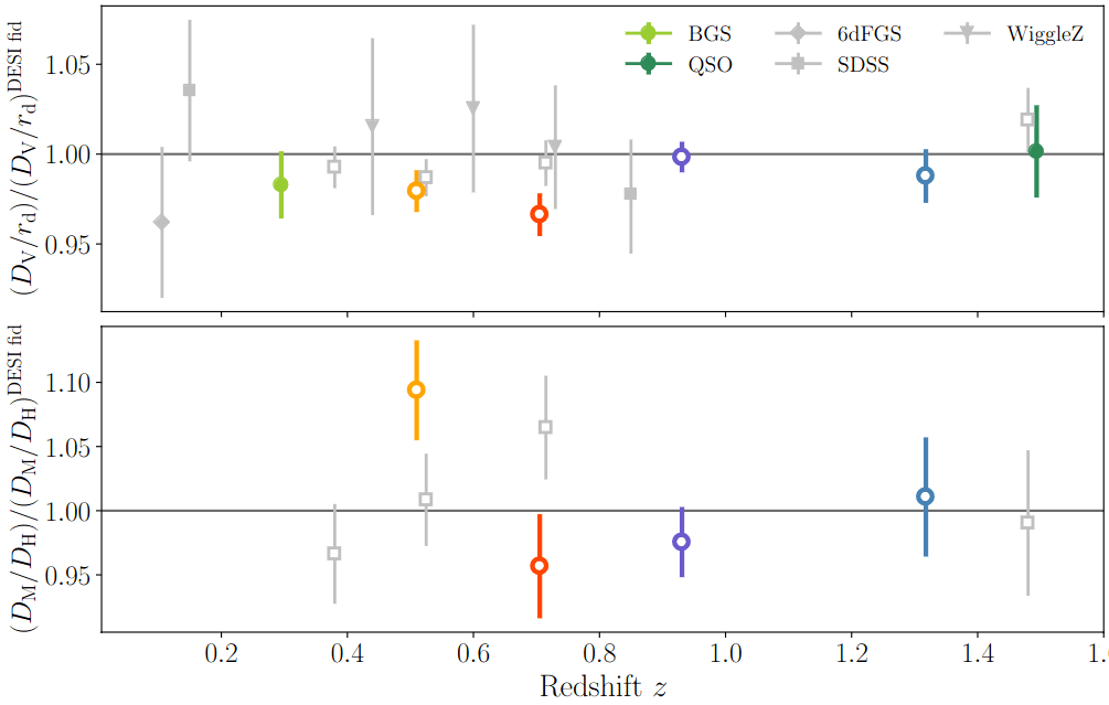
6dFGRS
SDSS (MGS)
SDSS (BOSS/eBOSS)
WiggleZ


\alpha_\mathrm{iso} \propto D_\mathrm{V}(z) / r_\mathrm{d} = (z D_{\mathrm{M}}^{2}(z) D_\mathrm{H}(z))^{1/3} / r_\mathrm{d}
\alpha_\mathrm{AP}^{-1} \propto D_\mathrm{M}(z) / D_\mathrm{H}(z)
\propto (D_{\mathrm{M}}^{2}(z) D_\mathrm{H}(z))^{1/3} / r_\mathrm{d} = f(\Omega_\mathrm{m}) / (H_0 r_\mathrm{d})
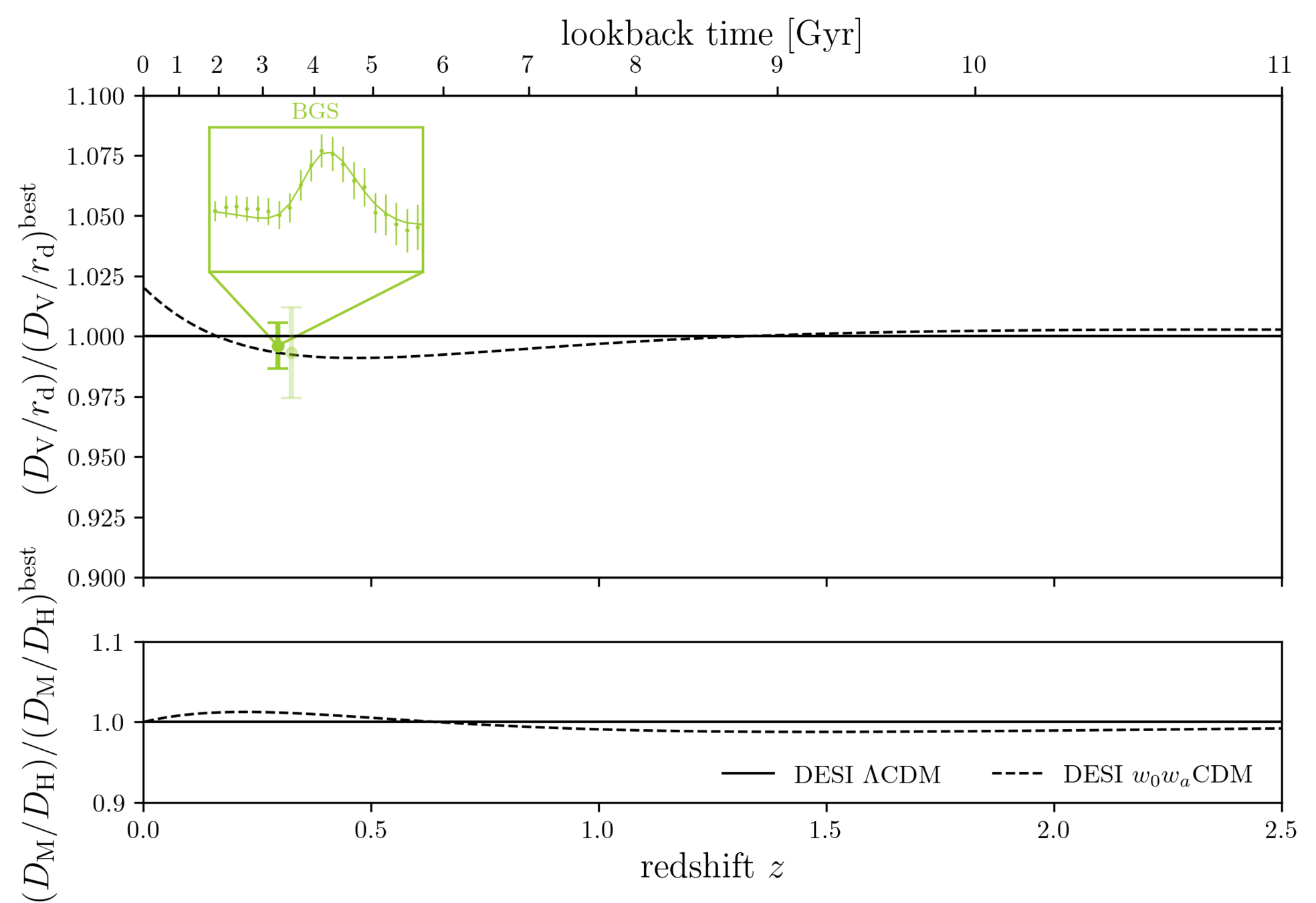
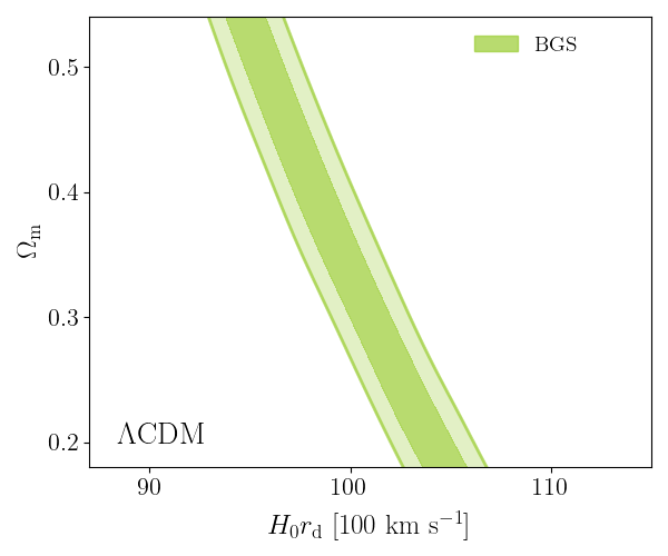
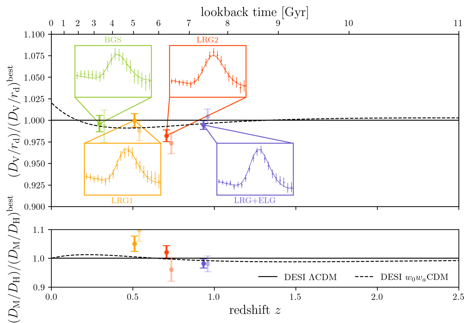
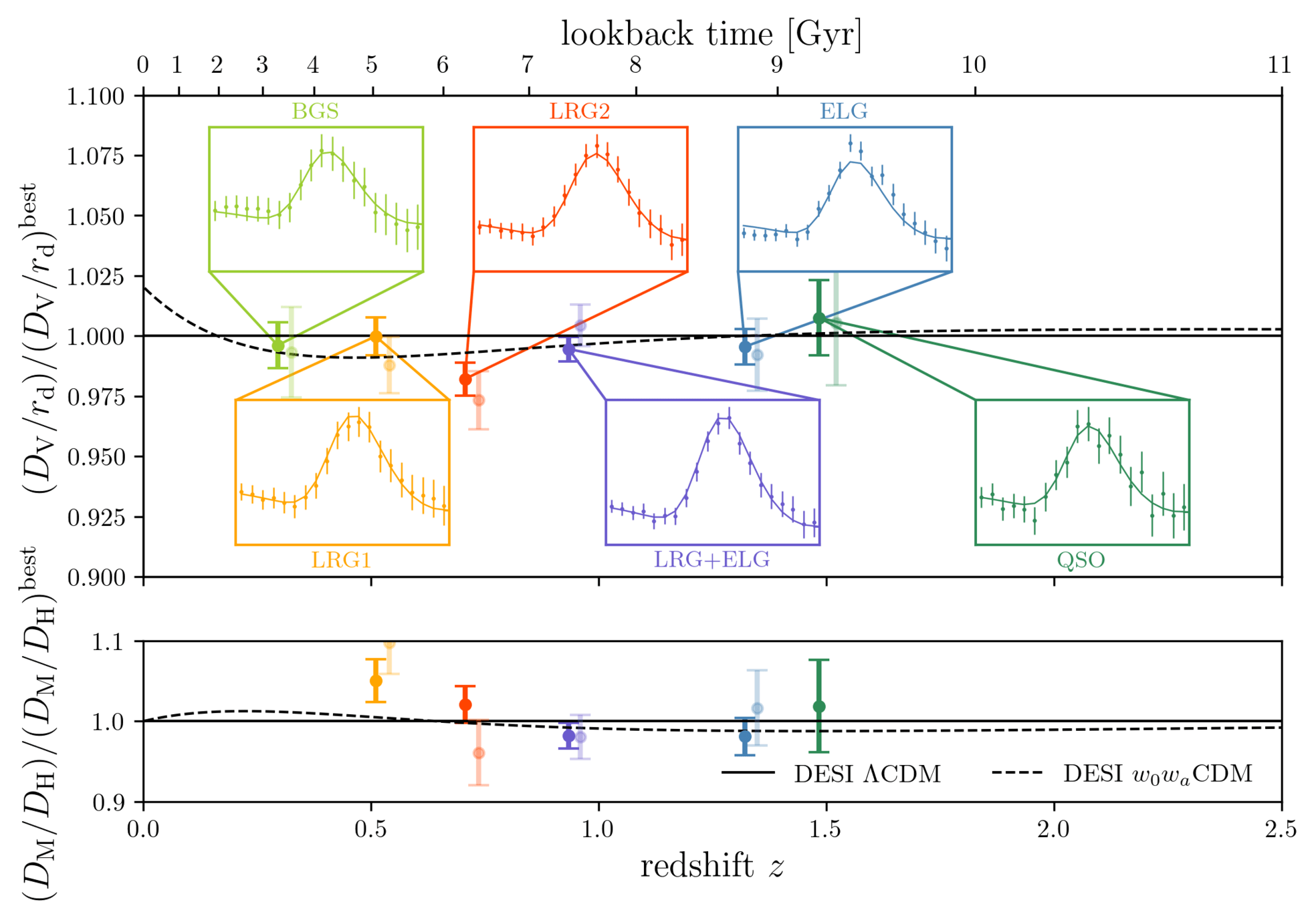
DESI DR2 BAO
\alpha_\mathrm{iso} \propto (D_{\mathrm{M}}^{2}(z) D_\mathrm{H}(z))^{1/3} / r_\mathrm{d} = f(\Omega_\mathrm{m}) / (H_0 r_\mathrm{d})
\orange{D_c(z)} = \int_0^z \frac{c dz^\prime}{\green{H(z^\prime)}} \qquad \text{with} \qquad \green{H(z)} = \purple{H_0} \sqrt{\blue{\Omega_\mathrm{m}} (1 + z)^3 + 1 - \Omega_\mathrm{m}}
Reminder:
\propto (D_{\mathrm{M}}^{2}(z) D_\mathrm{H}(z))^{1/3} / r_\mathrm{d} = f(\Omega_\mathrm{m}) / (H_0 r_\mathrm{d})
\propto \alpha_\mathrm{AP}^{-1} = (D_{\mathrm{M}}(z) / D_\mathrm{H}(z)) = f(\Omega_\mathrm{m})
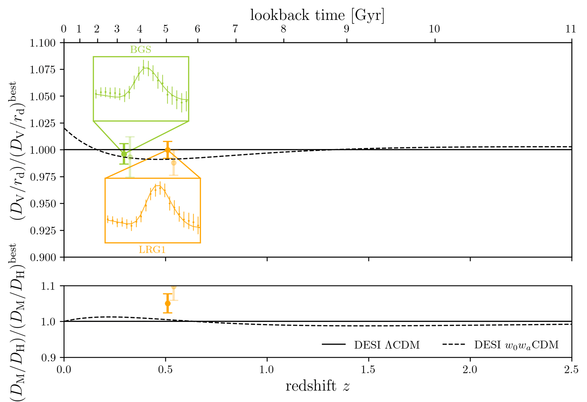
DESI DR2 BAO
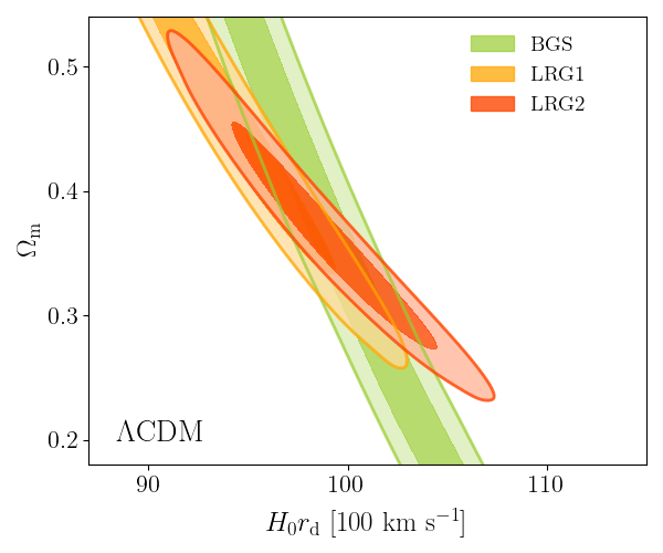
\propto (D_{\mathrm{M}}^{2}(z) D_\mathrm{H}(z))^{1/3} / r_\mathrm{d} = f(\Omega_\mathrm{m}) / (H_0 r_\mathrm{d})
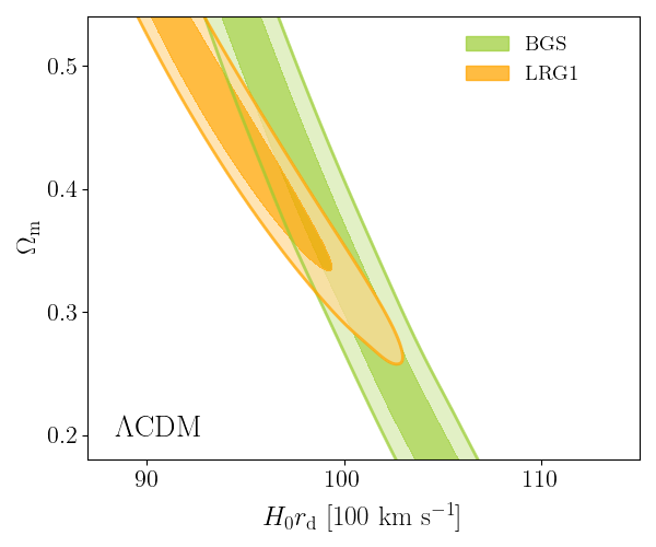
DESI DR2 BAO
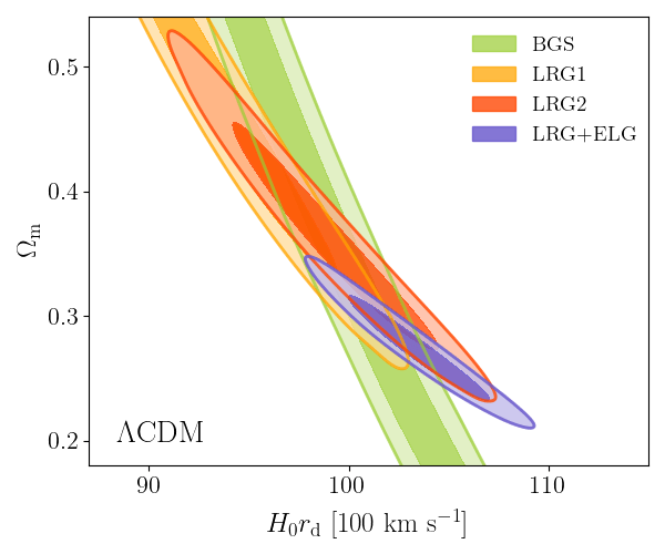
\propto (D_{\mathrm{M}}^{2}(z) D_\mathrm{H}(z))^{1/3} / r_\mathrm{d} = f(\Omega_\mathrm{m}) / (H_0 r_\mathrm{d})
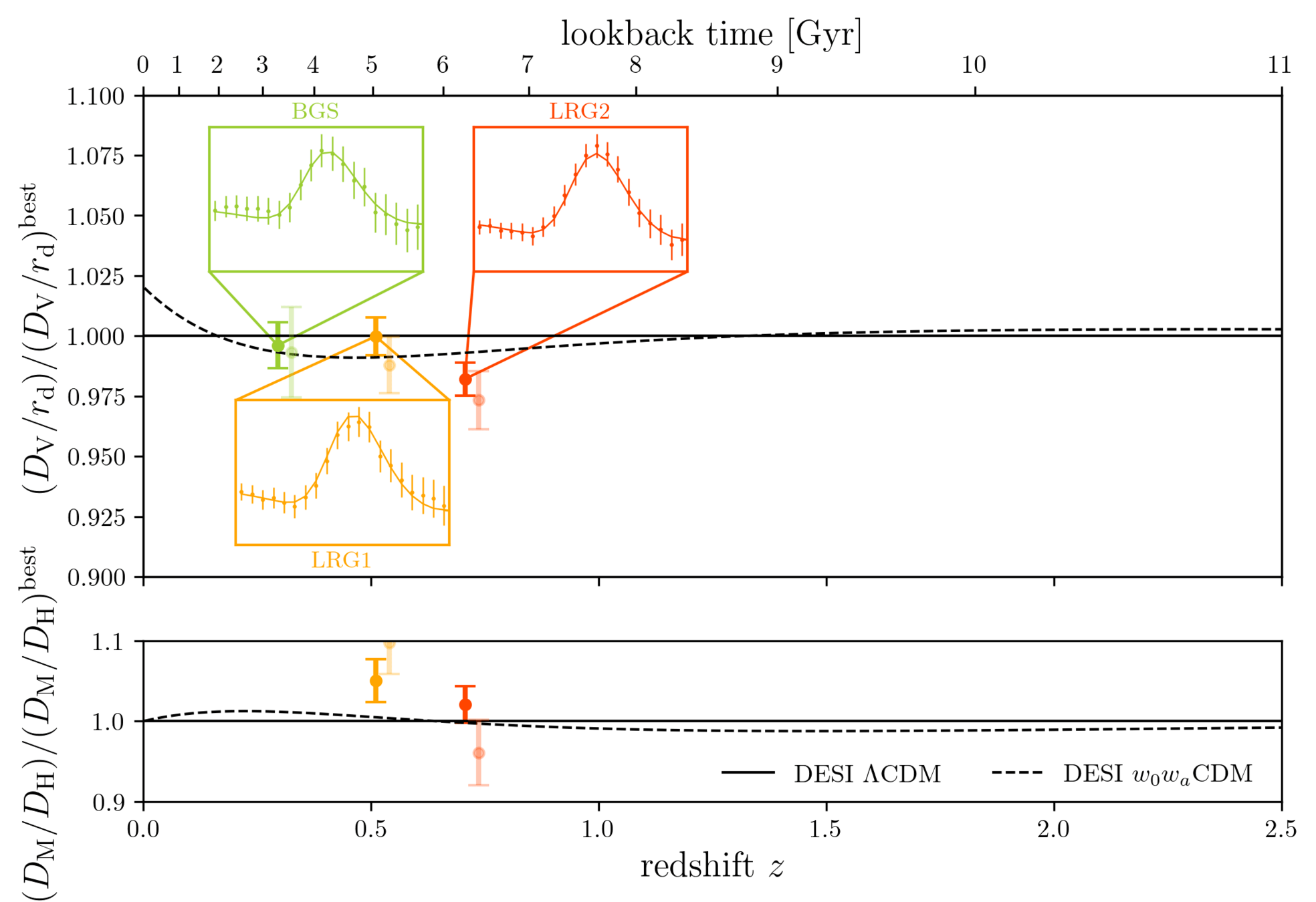
DESI DR2 BAO

\propto (D_{\mathrm{M}}^{2}(z) D_\mathrm{H}(z))^{1/3} / r_\mathrm{d} = f(\Omega_\mathrm{m}) / (H_0 r_\mathrm{d})
DESI DR2 BAO
\propto (D_{\mathrm{M}}^{2}(z) D_\mathrm{H}(z))^{1/3} / r_\mathrm{d} = f(\Omega_\mathrm{m}) / (H_0 r_\mathrm{d})
DESI DR2 BAO

\propto (D_{\mathrm{M}}^{2}(z) D_\mathrm{H}(z))^{1/3} / r_\mathrm{d} = f(\Omega_\mathrm{m}) / (H_0 r_\mathrm{d})
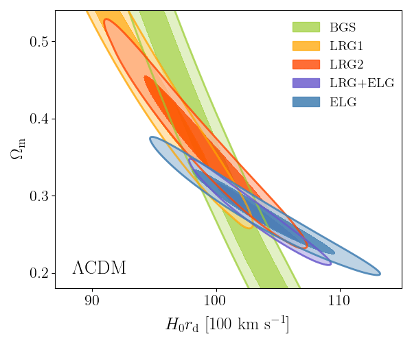
DESI DR2 BAO
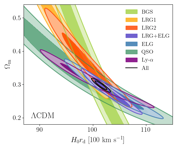
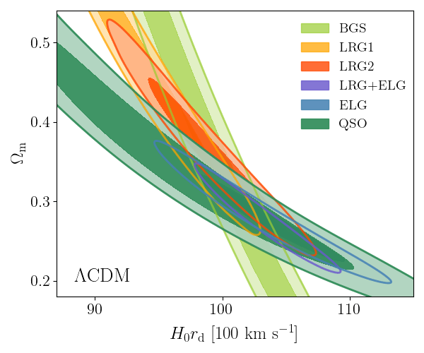
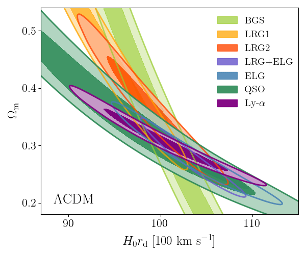
DESI DR2 BAO
Consistent with each other,
and complementary
\underbrace{\begin{align*}
\Omega_\mathrm{m} &= 0.2975 \pm 0.0086 & \mathbf{(3.0\%)} \\
H_{0} r_\mathrm{d} &= (101.54 \pm 0.73) \, [100 \, \mathrm{km} \, \mathrm{s}^{-1}] & \mathbf{(0.7\%)}
\end{align*}}_{\textstyle \text{\color{black}{DESI}}}
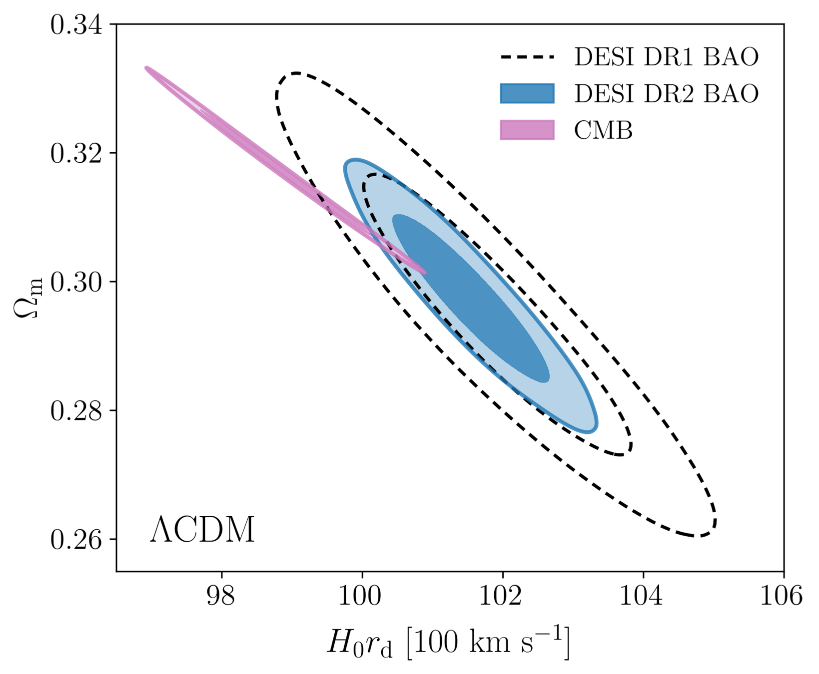
1. Planck PR4 CamSpec
2. Planck PR4 + ACT DR6 lensing
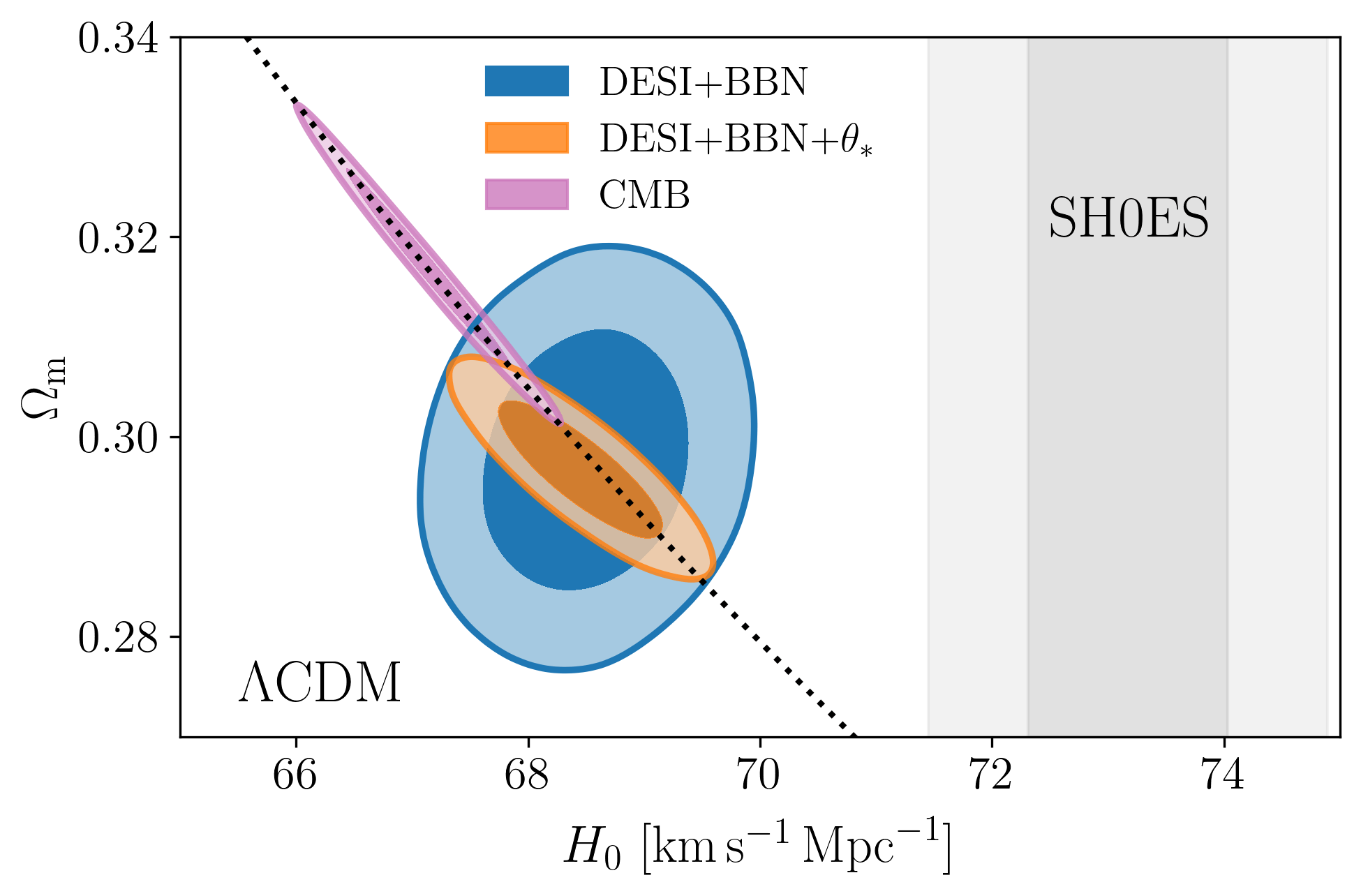
DESI DR2 BAO
- BAO constrains \(\Omega_\mathrm{m}\), \(h \times r_d(\Omega_\mathrm{b}h^2, \Omega_\mathrm{m}h^2 - \Omega_\nu h^2)\)
- Calibrating BAO relative distance measurements using BBN \(\Omega_\mathrm{b} h^2\)
\underbrace{
H_0 = (68.51 \pm 0.58) \, {\rm km\,s^{-1}\,Mpc^{-1}}
}_{\textstyle \color{darkblue}{\text{DESI} + \text{BBN}}}
\underbrace{
H_0 = (68.45 \pm 0.47) \, {\rm km\,s^{-1}\,Mpc^{-1}}
}_{\textstyle \color{orange}{\text{DESI} + \theta_\ast + \text{BBN}}}
- Adding very precise CMB acoustic angular scale
- In \(4.5\sigma\) tension with SH0ES (Breuval+24) (independently of the CMB)
DESI DR2 BAO
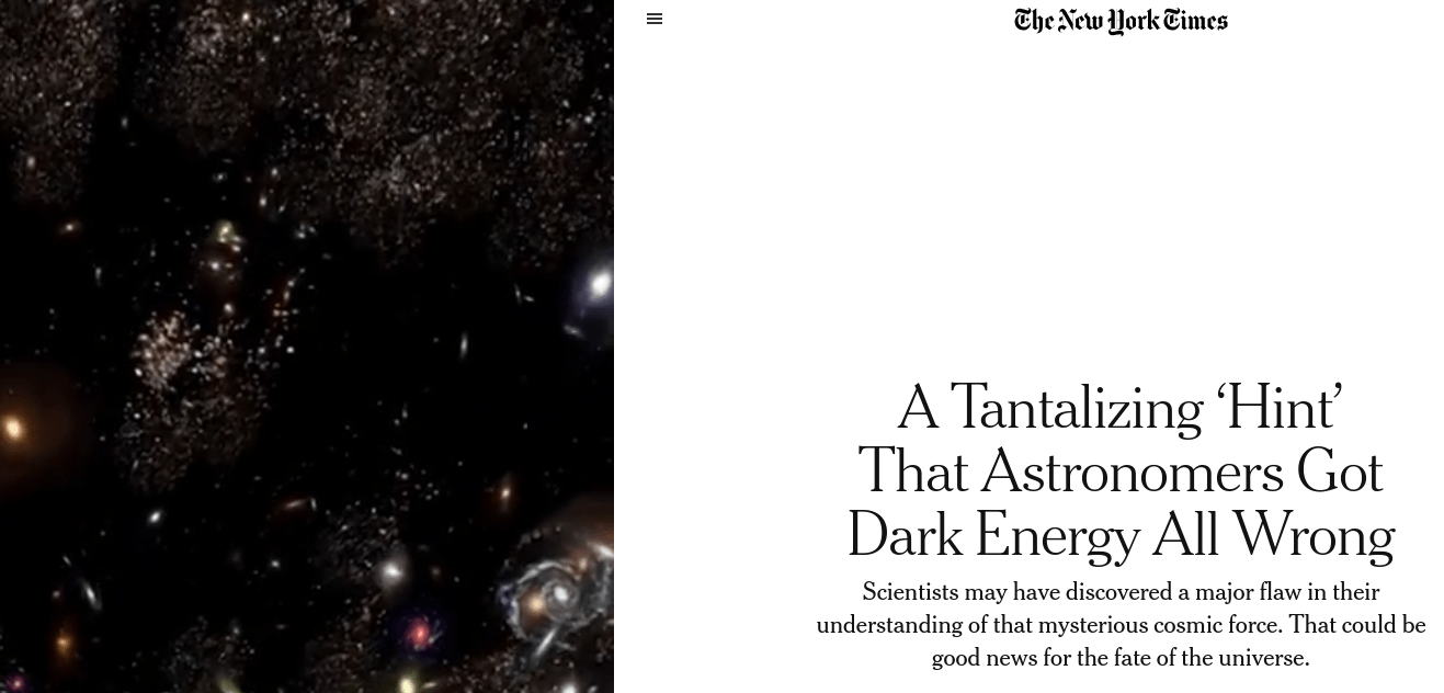
- Dark energy fluid
- No strong preference for dark energy evolution: \(1.7\sigma\) from DESI data alone
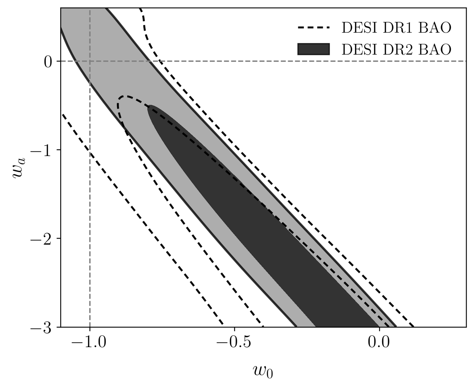
\(\Lambda\)
p / \rho = w = w_0 + w_a (1 - a)
pressure
density
CPL
DESI DR2 BAO
DESI DR2 BAO
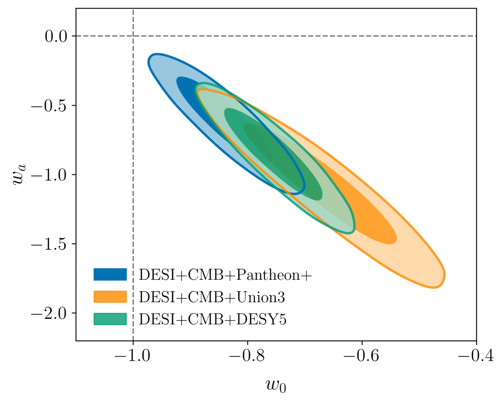
Combining all DESI + CMB + SN
\underbrace{
w_{0} = -0.838 \pm 0.055 \qquad w_{a} = -0.62^{+0.22}_{-0.19}
}_{\textstyle \textcolor{blue}{\text{DESI + CMB + Pantheon+} \; \implies \; 2.8\sigma}}
\underbrace{
w_{0} = -0.667 \pm 0.088 \qquad w_{a} = -1.09^{+0.31}_{-0.27}
}_{\textstyle \color{orange}{\text{DESI + CMB + Union3} \; \implies \; 3.8\sigma}}
\underbrace{
w_{0} = -0.752 \pm 0.057 \qquad w_{a} = -0.86^{+0.23}_{-0.20}
}_{\textstyle \color{green}{\text{DESI + CMB + DES-SN5YR} \; \implies \; 4.2\sigma}}
Internal CMB degeneracies limiting precision on the sum of neutrino masses
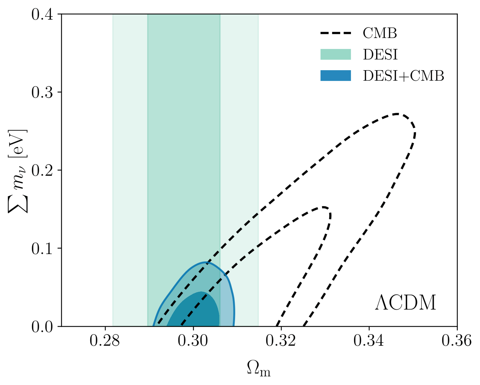
Broken by BAO, which favors low \(\Omega_\mathrm{m}\)
\sum m_\nu < 0.064 \, \mathrm{eV} \; (95\%, \text{DESI + CMB})
DESI DR2 BAO
Taken from Zhao et al. (2020)
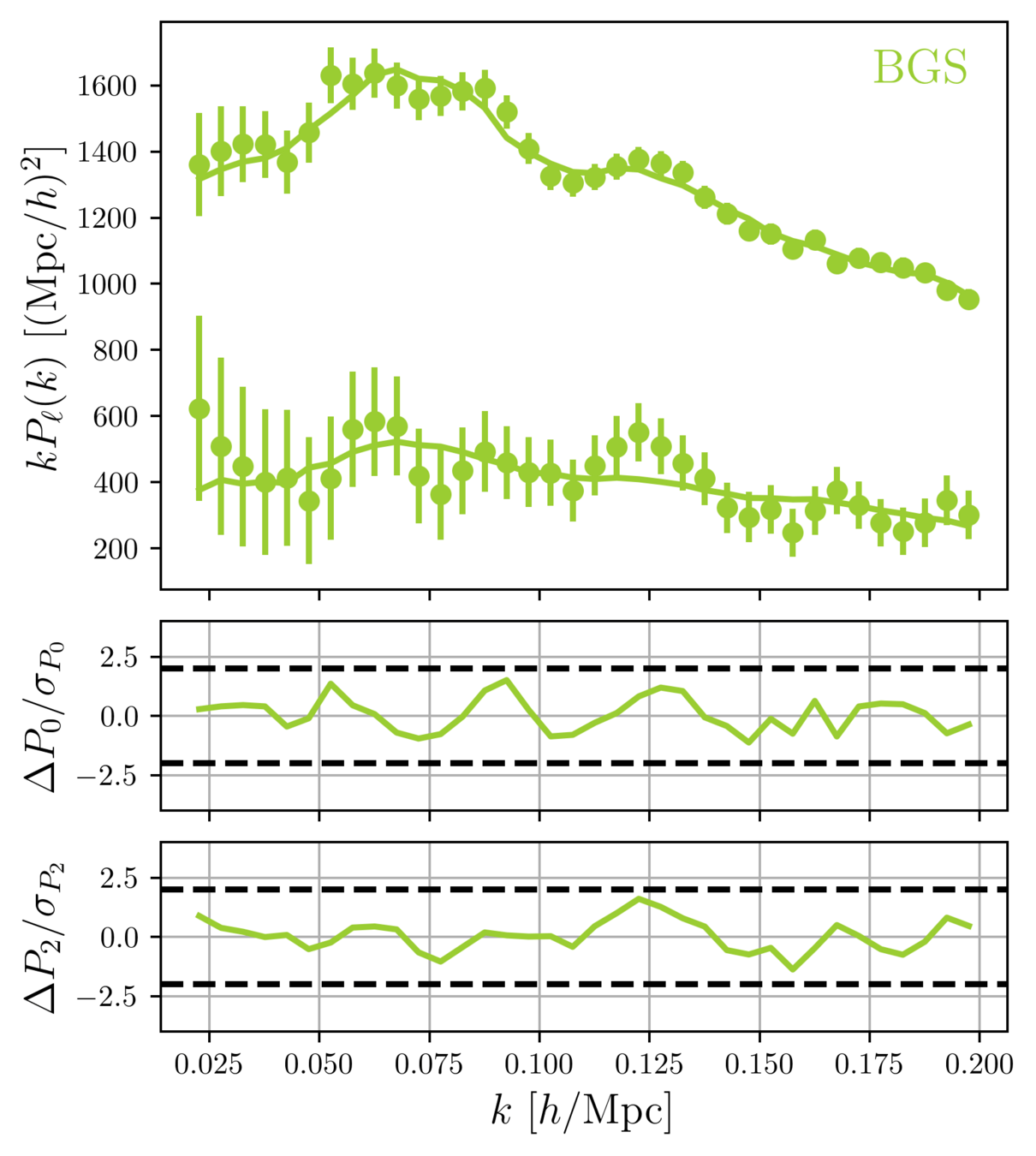
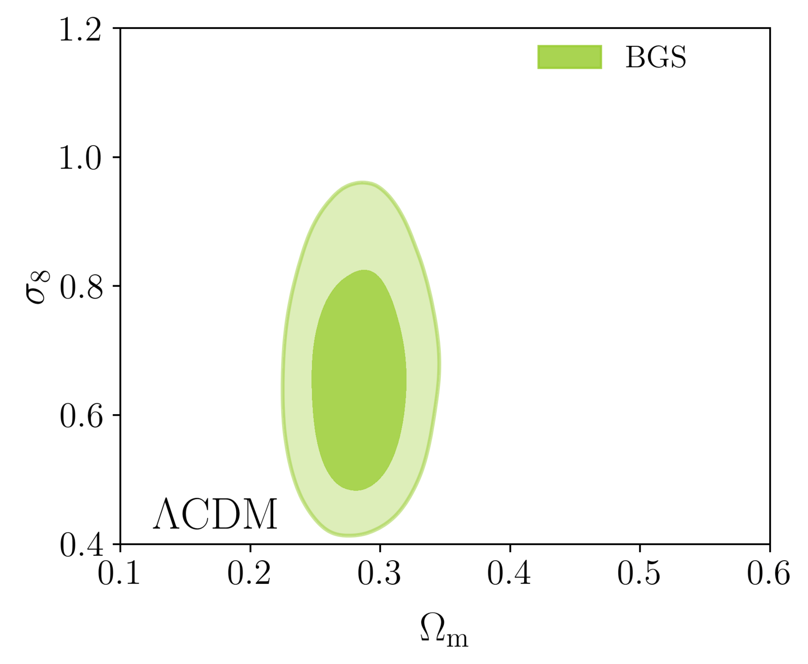
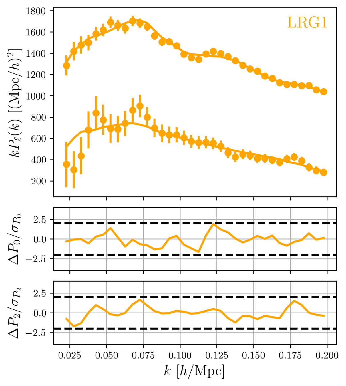
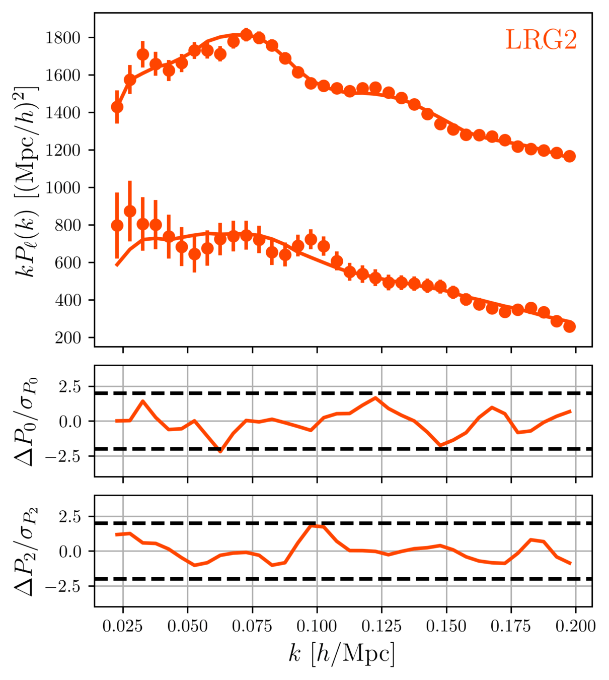
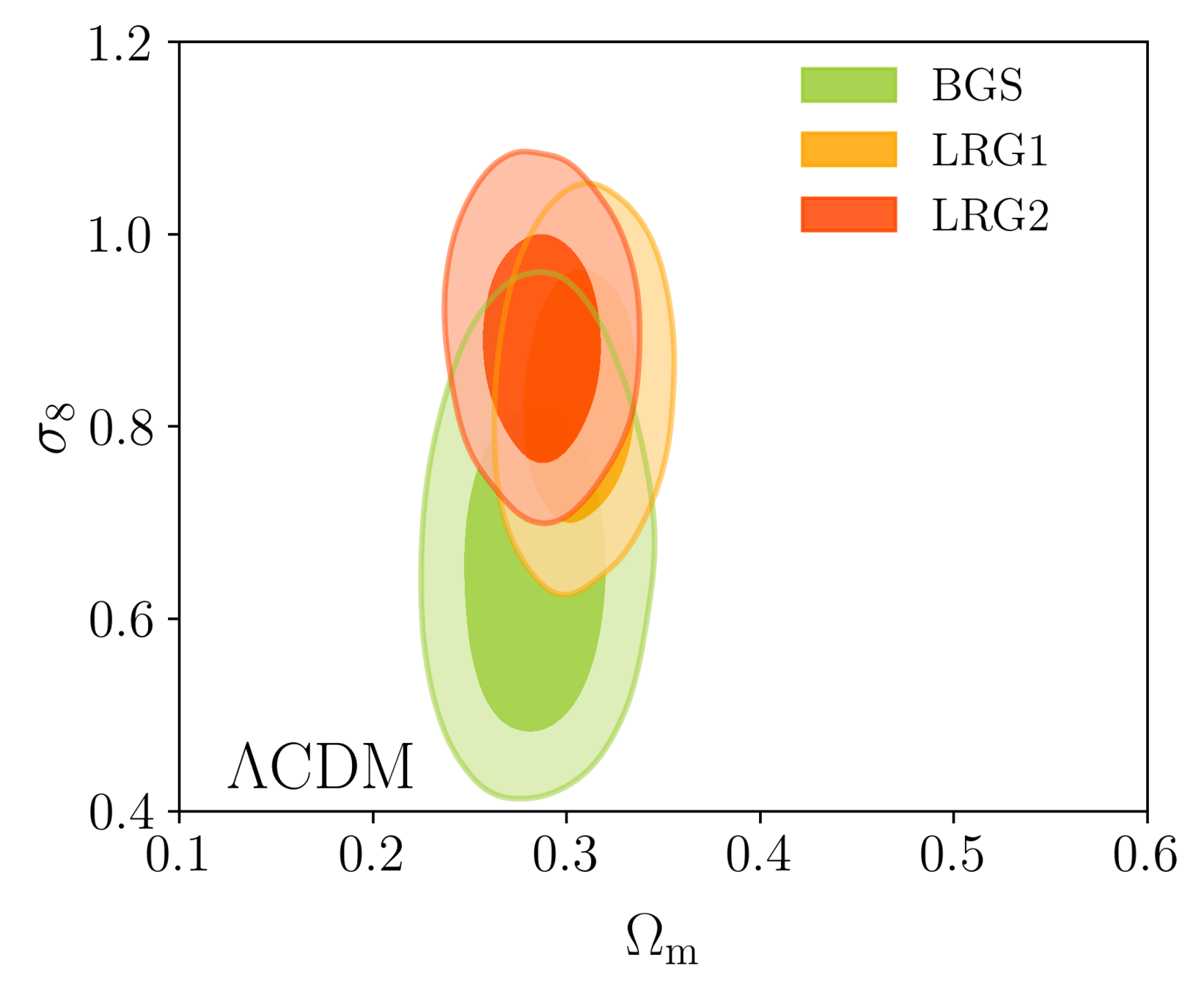
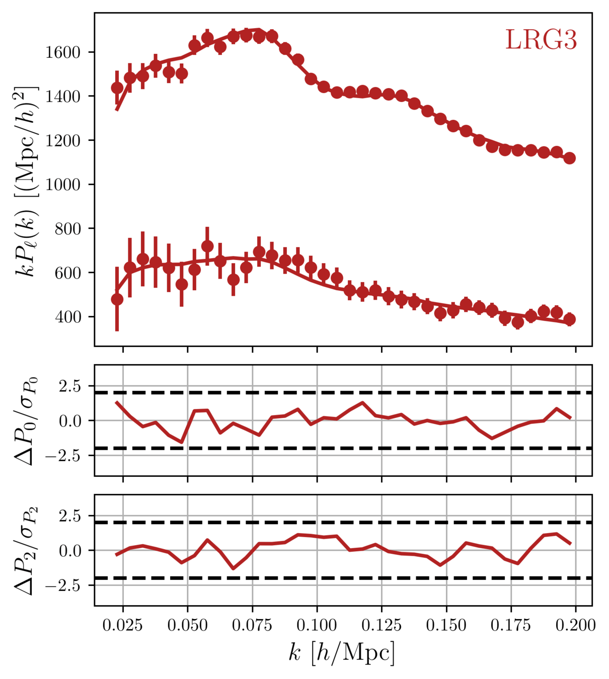
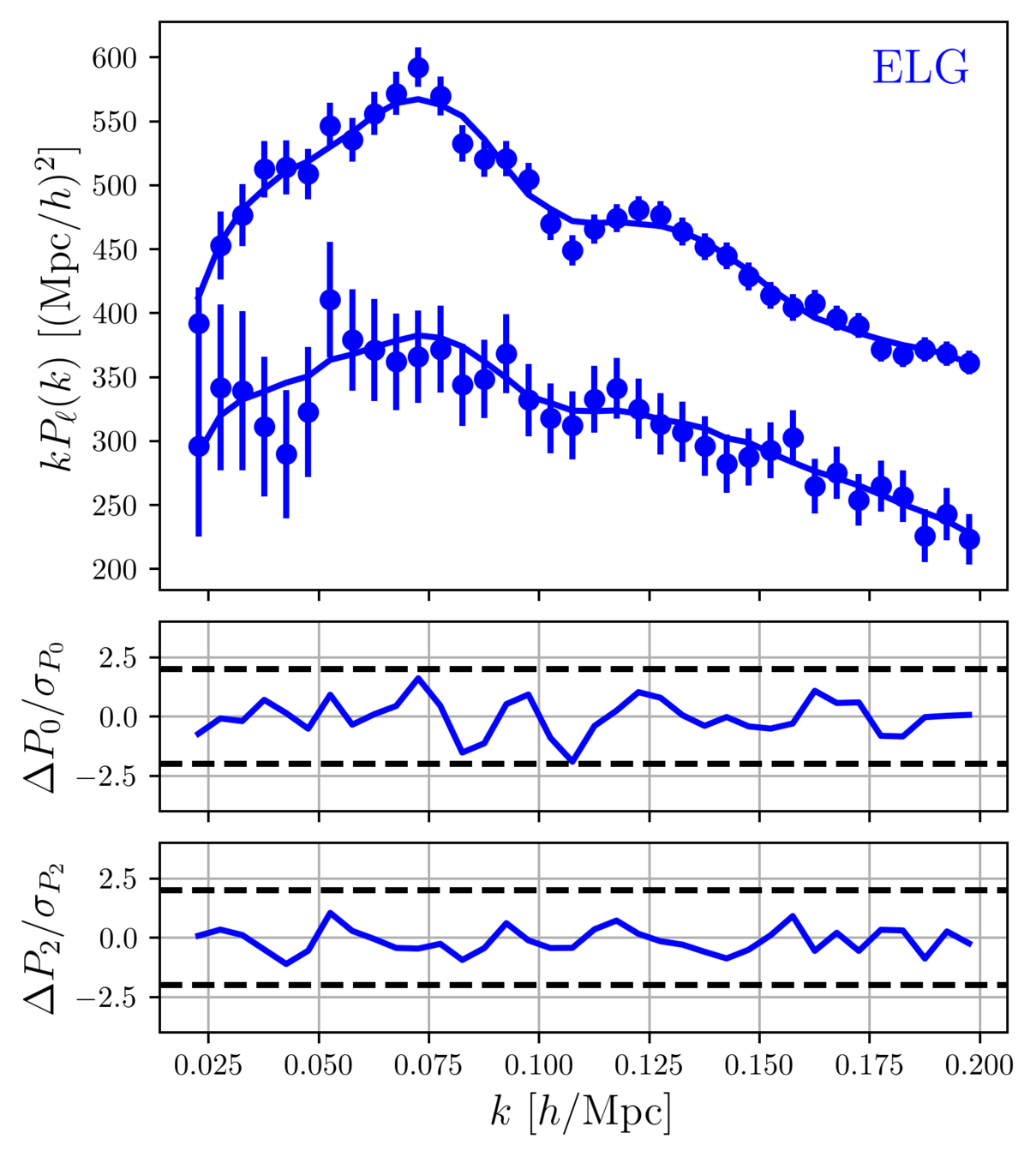
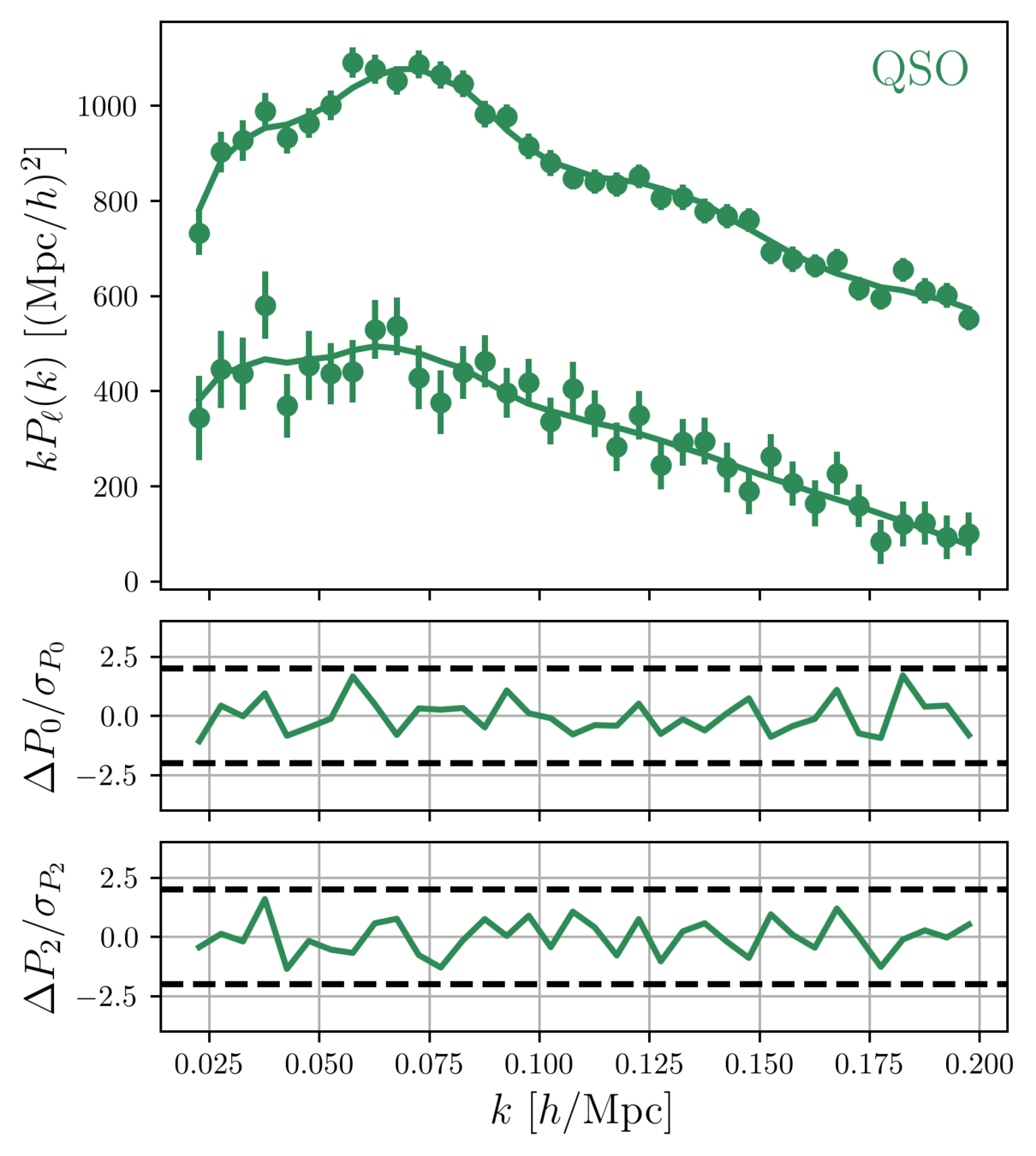
DESI DR1 Full Shape
DESI DR2 Full Shape results are not yet published! Come back next year ;) In the meantime, let's use DR1!
Taken from Zhao et al. (2020)
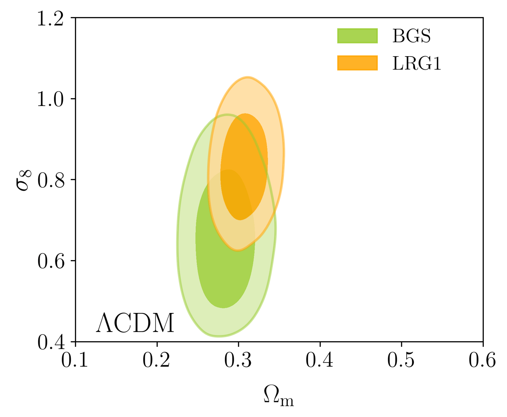
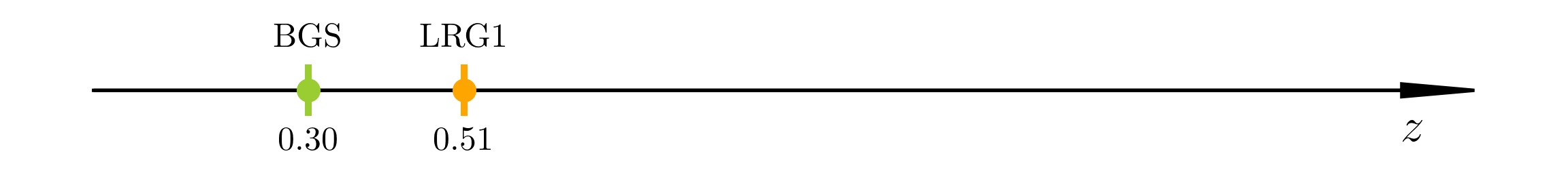
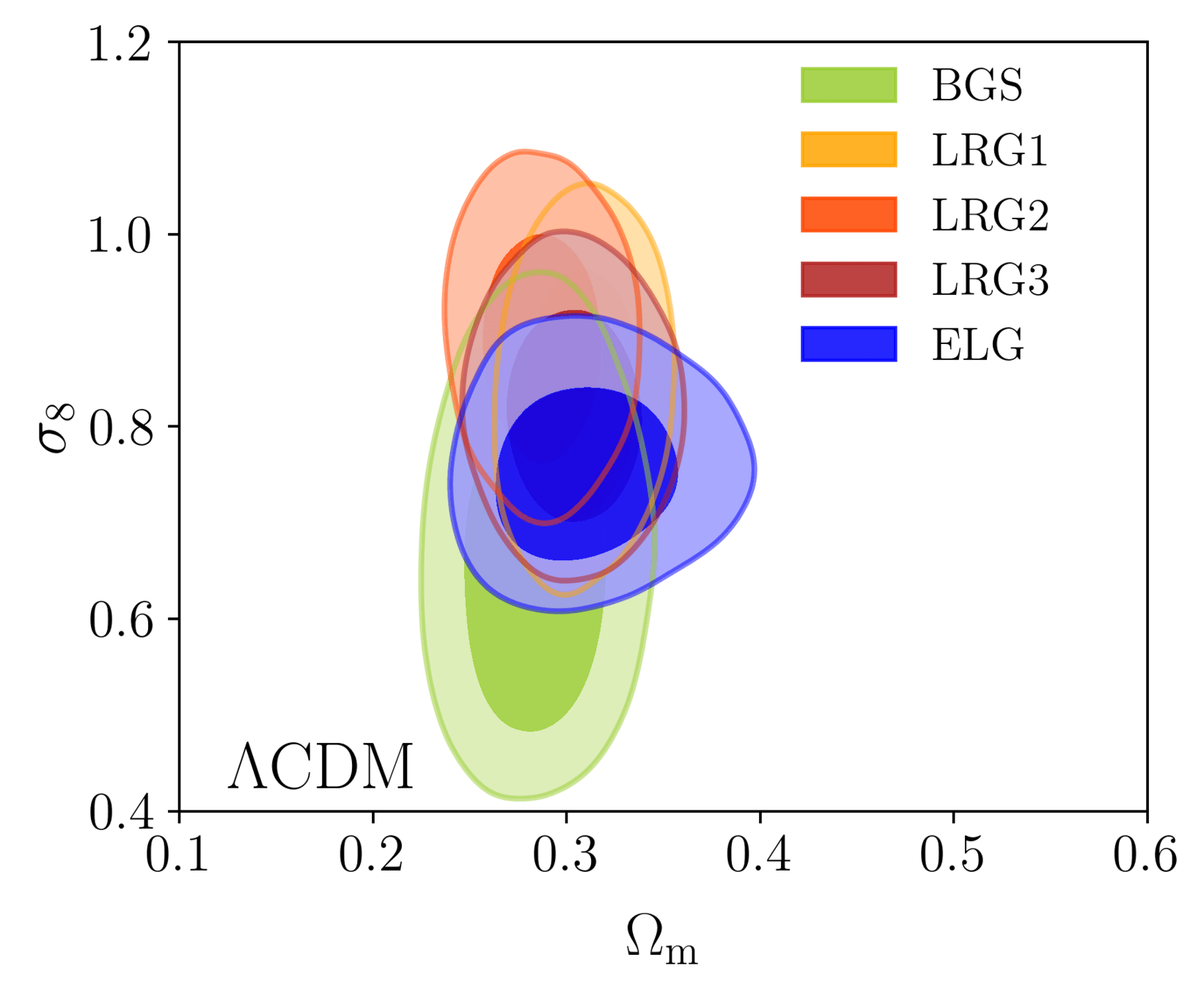
DESI DR1 Full Shape + BAO
\(\omega_\mathrm{b}\): BBN, \(n_\mathrm{s} \sim \mathcal{G}(0.9649, 0.042^2)\)
Taken from Zhao et al. (2020)
DESI DR1 Full Shape + BAO
\(\omega_\mathrm{b}\): BBN, \(n_\mathrm{s} \sim \mathcal{G}(0.9649, 0.042^2)\)
Taken from Zhao et al. (2020)
DESI DR1 Full Shape + BAO
\(\omega_\mathrm{b}\): BBN, \(n_\mathrm{s} \sim \mathcal{G}(0.9649, 0.042^2)\)
Taken from Zhao et al. (2020)
DESI DR1 Full Shape + BAO
\(\omega_\mathrm{b}\): BBN, \(n_\mathrm{s} \sim \mathcal{G}(0.9649, 0.042^2)\)
Taken from Zhao et al. (2020)
DESI DR1 Full Shape + BAO
\(\omega_\mathrm{b}\): BBN, \(n_\mathrm{s} \sim \mathcal{G}(0.9649, 0.042^2)\)
Taken from Zhao et al. (2020)
DESI DR1 Full Shape + BAO
\(\omega_\mathrm{b}\): BBN, \(n_\mathrm{s} \sim \mathcal{G}(0.9649, 0.042^2)\)
Taken from Zhao et al. (2020)
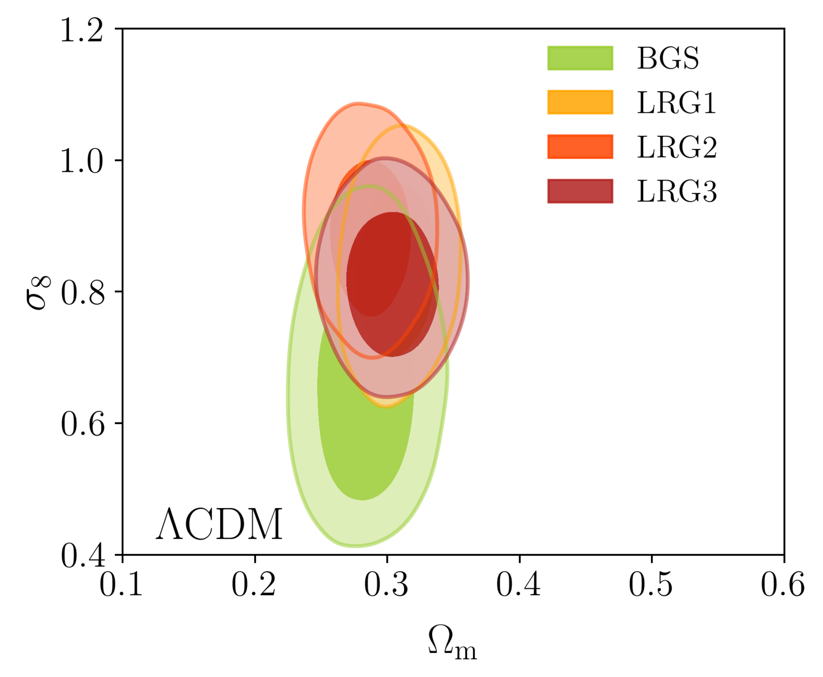
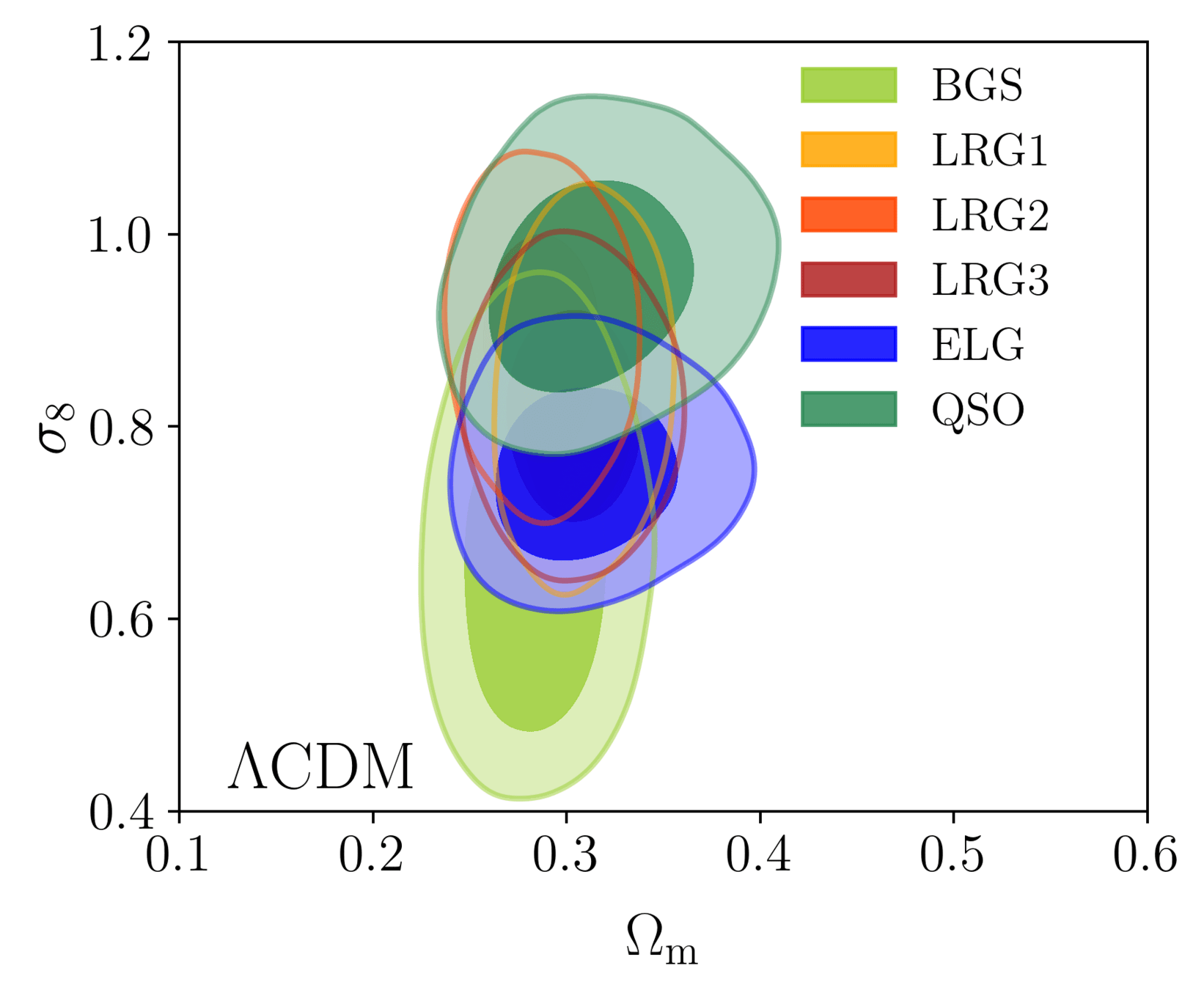
- Consistency with SDSS
- In agreement with CMB
- Weak lensing prefers lower \(S_8\), but still consistent
- FS measurement competitive with weak lensing
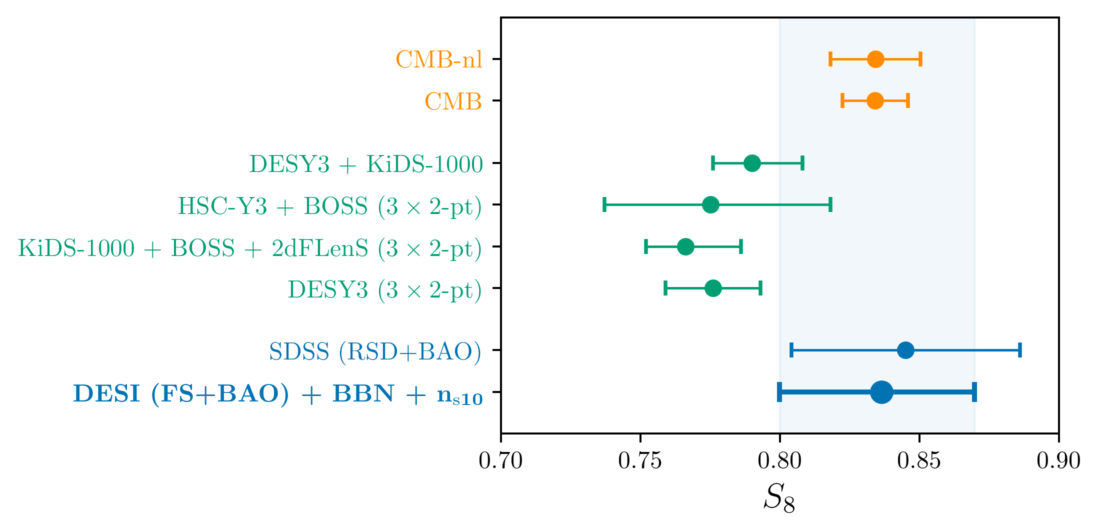
\(S_8 = \sigma_8 (\Omega_\mathrm{m} / 0.3)^{0.5}\) best constrained by weak lensing surveys
\underbrace{
S_8 = 0.836 \pm 0.035
}_{\textstyle \text{\color{blue}{DESI + BBN + $n_{s10}$}}}
DESI DR1 Full Shape + BAO
Taken from Zhao et al. (2020)
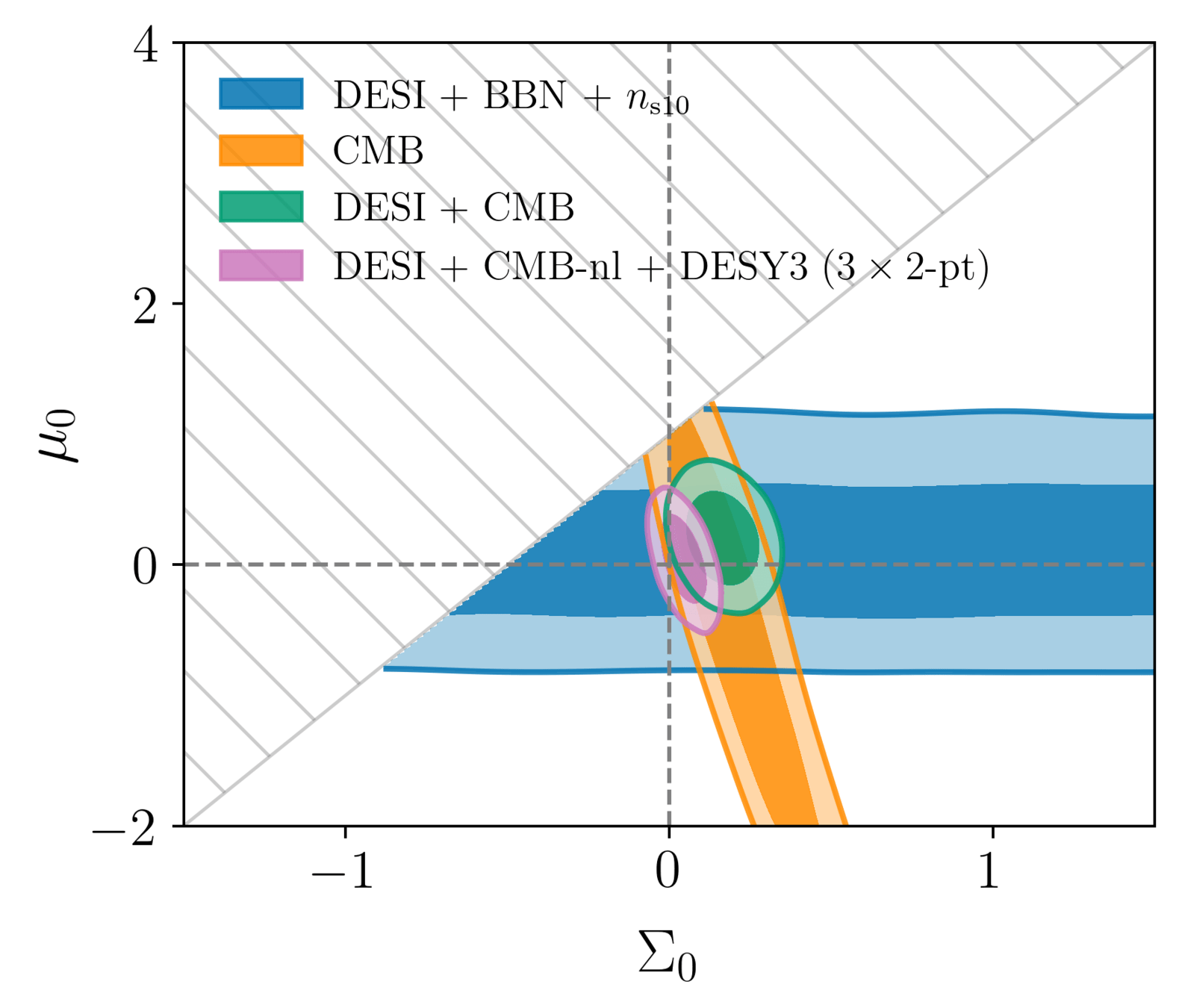
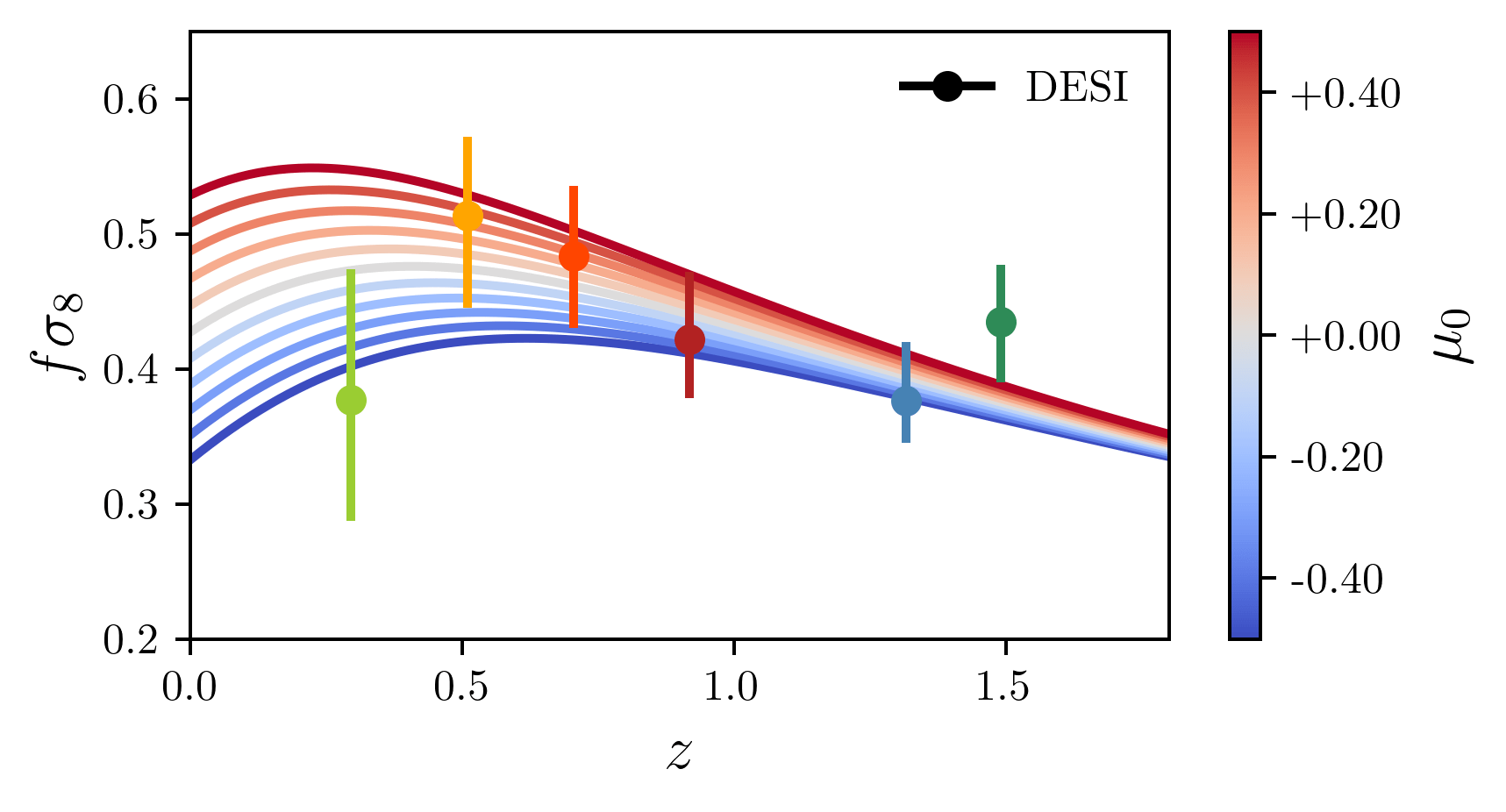
Modified gravity constraints
In general relativity, \(\green{\mu(a, k)} = \green{\Sigma(a, k)} = 1\)
To test GR, introduce \(\green{\mu_0, \Sigma_0}\)
\mu(a) = 1 + \frac{\Omega_\Lambda(a)}{\Omega_\Lambda} \green{\mu_0}, \Sigma(a) = 1 + \frac{\Omega_\Lambda(a)}{\Omega_\Lambda} \green{\Sigma_0}
Perturbed FLRW metric
\(ds^2=a(\tau)^2[-(1+2\orange{\Psi})d\tau^2+(1-2\orange{\Phi})\delta_{ij}dx^i dx^j]\)
At late times:
(mass) \(k^2\orange{\Psi} = -4\pi G a^2 \green{\mu(a,k)} \blue{\sum_i\rho_i\Delta_i}\)
(light) \(k^2(\orange{\Phi} + \orange{\Psi})=-8\pi G a^2 \green{\Sigma(a,k)} \blue{\sum_i\rho_i\Delta_i}\)
gravitational potentials
density perturbations
Taken from Zhao et al. (2020)
\(\Sigma_0\) constrained by
- CMB (ISW and lensing)
- galaxy lensing
\underbrace{\begin{align*}
\mu_0 &= 0.04\pm 0.22 \\
\Sigma_0 &= 0.045\pm 0.046
\end{align*}}_{\textstyle \text{\color{purple}{DESI + CMB-nl + DESY3 ($3\times 2$-pt)}}}

\underbrace{
\mu_0 = 0.11^{+0.45}_{-0.54}
}_{\textstyle \text{\color{blue}{DESI + BBN + $n_{\mathrm{s}10}$}}}
compared to CMB-nl + DESY3 (3x2pt) only: \(\sigma(\mu_0) / 2.5\), \(\sigma(\Sigma_0) / 2\)
DESI constrains
Modified gravity constraints
Taken from Zhao et al. (2020)
Cosmological constraints - take aways
BAO
- constrains distances / the Hubble rate \(\Rightarrow\) energy content
- compared to Planck: low \(\Omega_\mathrm{m}\), high \(H_{0}\)
- hint of dynamical dark energy (depending on SN dataset)
Adding Full Shape
- probes structure growth
- \(\sigma_8, S_8\) consistent with Planck
- modified gravity parameter \(\mu_0\) consistent with GR
Primordial non-Gaussianity (left by inflation):
- scale-dependent bias \(\propto k^{-2}\)
- consistent with 0: \(f_\mathrm{NL}^\mathrm{loc} = -3.6^{+9.0}_{-9.1}\) (Chaussidon et al. 2024)
Taken from Zhao et al. (2020)
Other clustering analyses
- higher order correlation functions (3-pt, 4-pt...): e.g. Slepian et al. 2017, Hou et al. 2022, Philcox et al. 2022
- alternative clustering statistics: e.g. density-split correlation function, 1D PDF, Wavelet Scattering Transforms, neural compression, e.g. Paillas et al. 2023, Beyond-2pt collaboration, Lemos et al. 2023
- field-level inference of the galaxy density, e.g. Lavaux et al. 2019
- cross-correlations: galaxy clustering x galaxy weak lensing, e.g. Chen et al. 2024, galaxy clustering x CMB weak lensing Sailer et al. 2024
- continuous tracer Ly\(\alpha\): probe HI density along line-of-sight ⇒ BAO DESI 2025, P1D Ravoux et al. 2025
- photometric surveys: BAO with DES Collaboration et al. 2025, Vera Rubin (LSST)
LSS formation galaxy bias
truth
samples
Taken from Zhao et al. (2020)
Other clustering analyses
- higher order correlation functions (3-pt, 4-pt...): e.g. Slepian et al. 2017, Hou et al. 2022, Philcox et al. 2022
- alternative clustering statistics: e.g. density-split correlation function, 1D PDF, Wavelet Scattering Transforms, neural compression, e.g. Paillas et al. 2023, Beyond-2pt collaboration, Lemos et al. 2023
- field-level inference of the galaxy density, e.g. Lavaux et al. 2019
- cross-correlations: galaxy clustering x galaxy weak lensing, e.g. Chen et al. 2024, galaxy clustering x CMB weak lensing Sailer et al. 2024
- continuous tracer Ly\(\alpha\): probe HI density along line-of-sight ⇒ BAO DESI 2025, P1D Ravoux et al. 2025
- photometric surveys: BAO with DES Collaboration et al. 2025, Vera Rubin (LSST)
Introduction_to_galaxy_clustering_2025
By Arnaud De Mattia


