Simulating AGN feedback
Arnau Quera-Bofarull
Supervised by: Cedric Lacey, Chris Done & Richard Bower
A study of AGN line-driven winds
What is AGN feedback?
Energy coupling between the central black hole and its host galaxy.
\frac{\text{size of BH}}{\text{size of Galaxy}} \approx

Joint evolution of BH and Galaxy
- This energy coupling implies a joint evolution between the black hole and the host galaxy.
-
BH mass is correlated with bulge luminosity and velocity dispersion across a wide range.
Kormendy and Ho (2013)
Black Hole Mass
Bulge velocity dispersion

Kormendy & Ho (2013)
Effects on galaxy population.
Image credit: Mutch et al (2013)
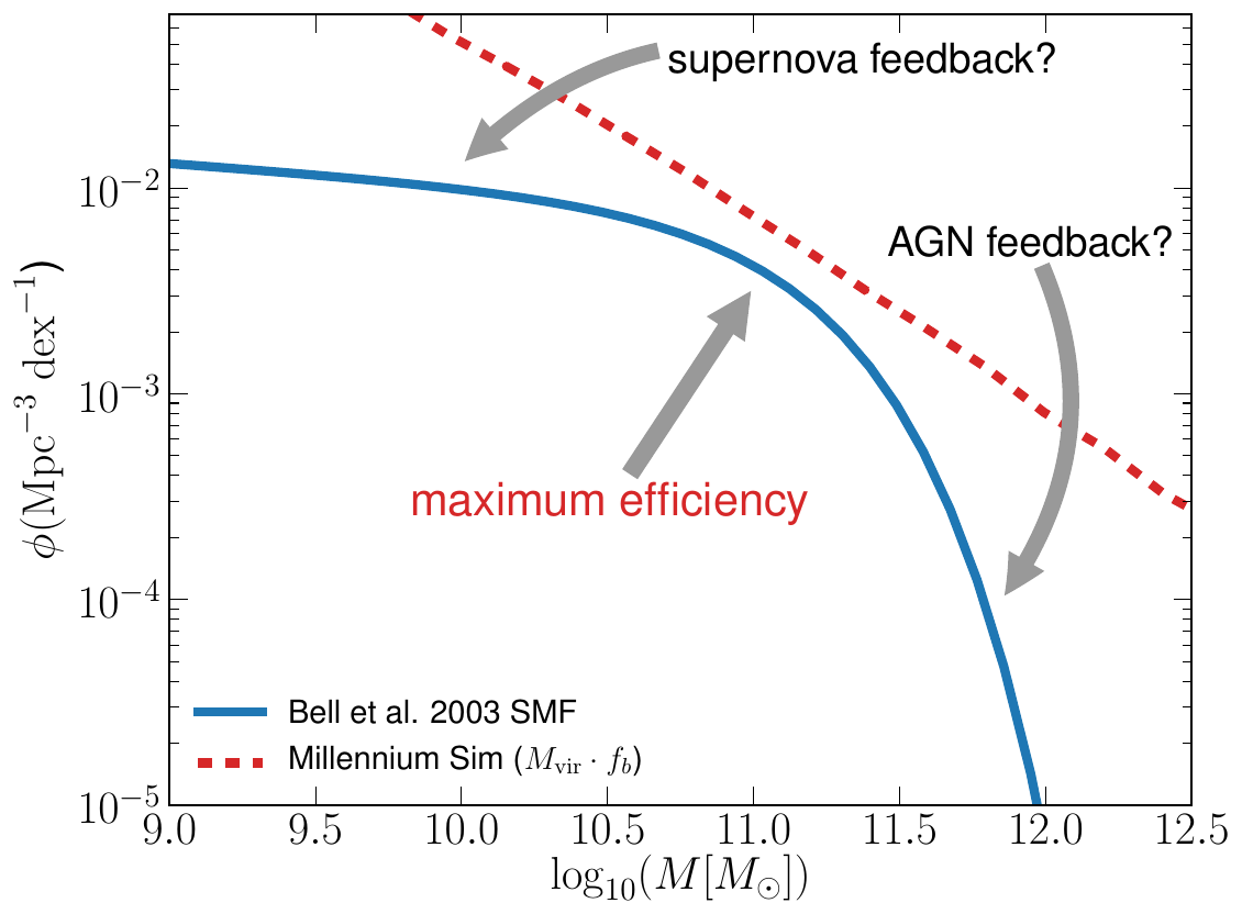
Mass
Mass Function
(log) Mass Number Count
Stellar Mass
Schaye et al (2014)
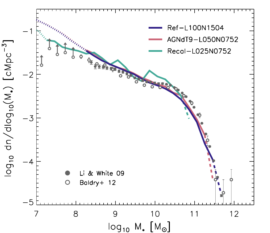
AGN ( and supernova) feedback are needed to match observations.
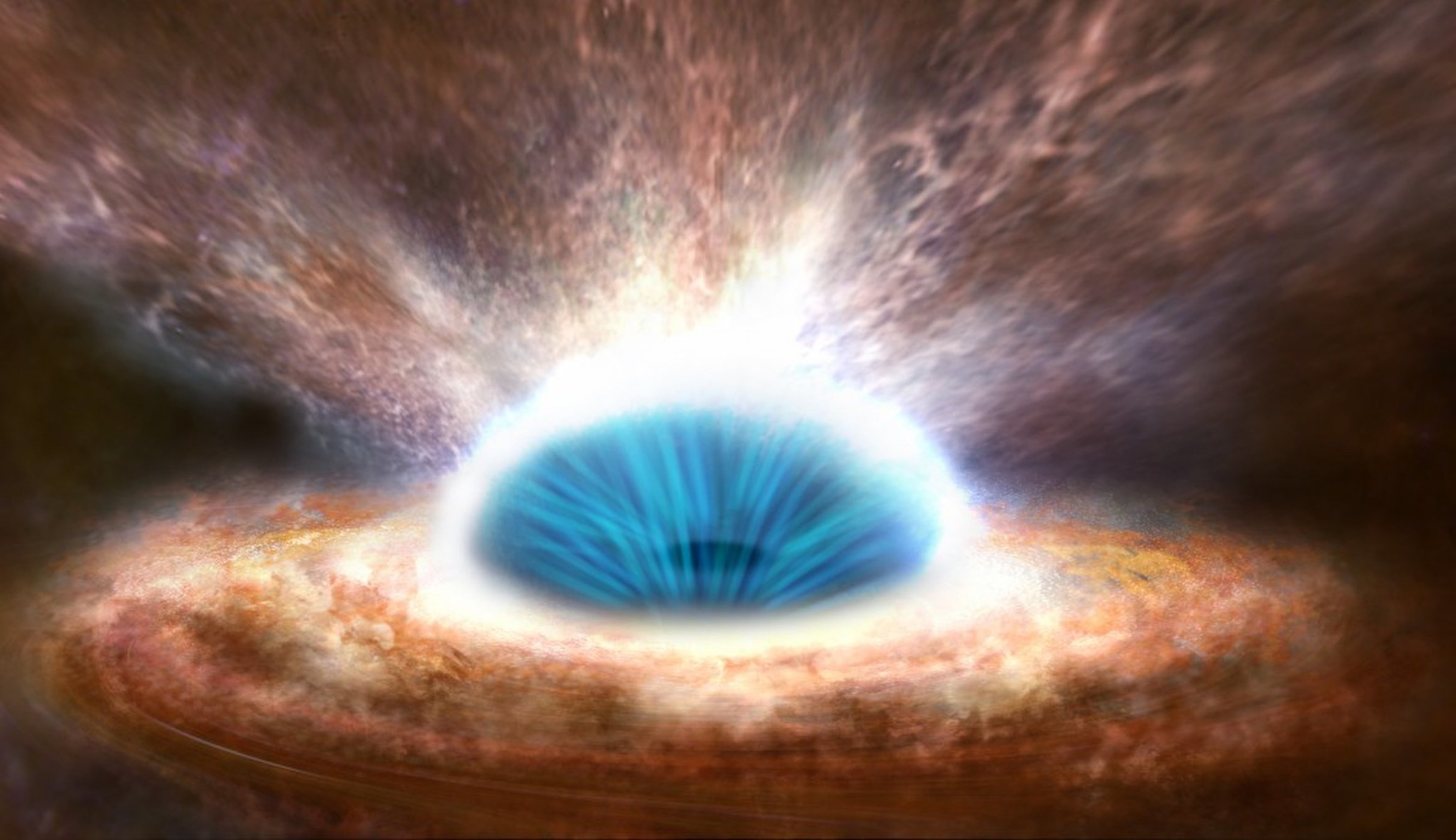
The origin of the coupling: Accretion
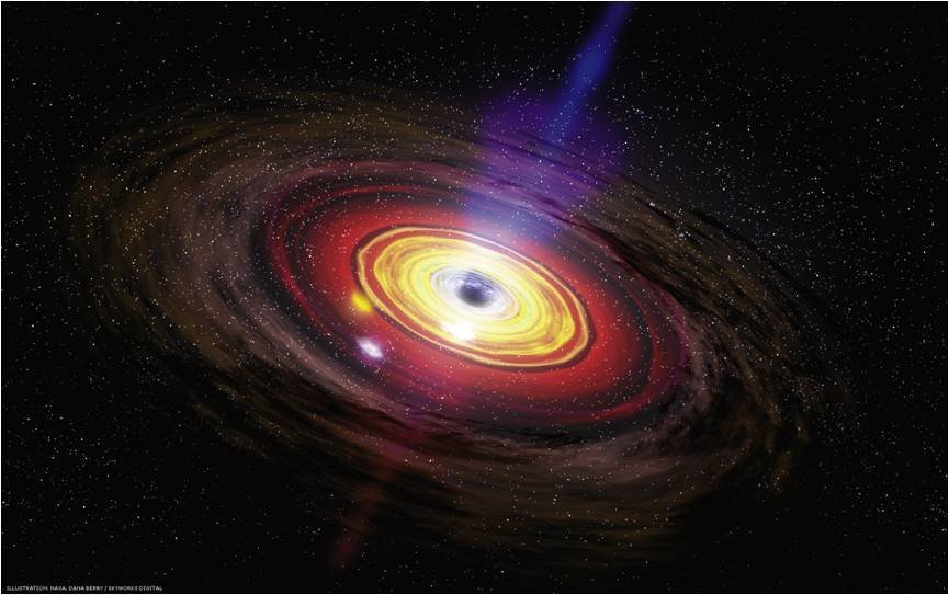
E = \eta m c^2
\text{ BH accretion } \rightarrow \eta \approx 0.1
Credit: NASA/Goddard Space Flight Center
- Matter falls in gaining kinetic energy.
- Part of this energy released as radiation.
Fun fact: throwing 50kg down to a black hole powers the UK electric grid for a year!
Is that enough to alter the galaxy?
E_\text{outflow} \approx 0.1 M_{BH} c^2 \approx 10^{61} \text{erg}
\text{Consider a BH grown through accretion to } M = 10^8 M_\odot
\text{Consider a galaxy bulge with } M=10^{11} M_\odot \text{ and } \sigma_v = 200 \text{km}/\text{s}
E_\text{binding} \approx M_\text{bulge} \sigma_v^2 \approx 10^{58} \text{erg}
More than enough energy...
Can this radiation be (minimally) coupled with the surrounding material?
Eagle AGN feedback
In EAGLE, a fraction of the radiated energy from accretion is coupled thermally to the surrounding gas.
\dot E_\text{inj} = \epsilon_f \dot E_\text{acc.}
Calibrated to match observations (ϵ = 0.15).
Since final BH masses depend on it, they are not a prediction of the simulation.
Ideally, ϵ should be derived from first principles.
\epsilon_f = \epsilon_f ( M_\text{BH}, \dot M, a)
Feedback mechanisms
Radiative mode
Kinetic mode
Winds
Credit: ESA/ATG medialab
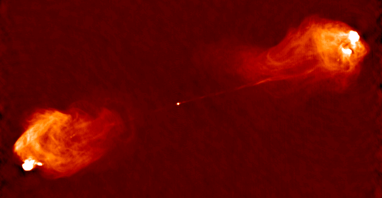
Credit: NRAO/AUI
\text{Unlikely to directly cause } M - \sigma \text{ relation.}
Jets
Radiation vs Gravity
The Eddington Limit
g_\text{rad} = g_\text{rad}\left( \kappa , L\right)
Luminosity
Opacity
g_\text{grav} = g_\text{grav}\left(M_\text{BH}\right)
\text{Assuming } \kappa = \kappa_{e.s.} \text{, both quantities are equal at }
L_\text{Edd} = \frac{4 \pi G M_\text{BH} c}{\kappa_\text{es}}
How do we create a wind?
L>L_\text{Edd} \longrightarrow \text{ Super Eddington winds}
\kappa > \kappa_\text{e.s.} \longrightarrow \text{Line-driven winds}
Radiation vs Gravity
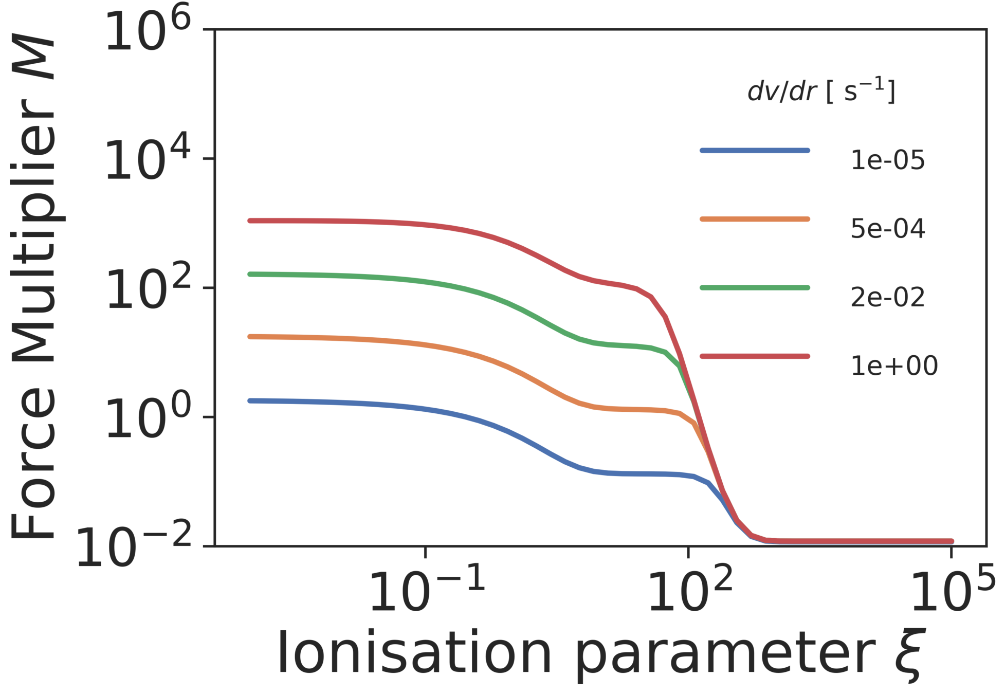
The line-driving mechanism
Opacities can be much larger than free electron scattering.
\frac{\kappa_\text{lines + e.s.}}{\kappa_\text{e.s}} = M\left( \frac{dv}{dr}, \xi \right)
v
\xi \propto L_\text{X-Rays}
Ionisation parameter
Castor, Abbot & Klein (1975)
Force Multiplier
The setup
Need to shield against X-Rays
How to drive a wind
X-Rays vs UV
- Need a shielding mechanism that sets ξ < 100 at ~ 100-400 Rg.
- Most of the work so far, e.g.,
- Proga & Kallman (2000, 2004)
- Risaliti & Elvis (2010)
- Nomura et al ( 2013, 2016, 2017, 2018)
\sigma_\text{X} = \begin{cases}
\sigma_\text{e.s.} & \text{ if } \xi > 10^5 \\
100\sigma_\text{e.s.} & \text{ if } \xi < 10^5
\end{cases}
assumes X-Ray opacities to be
Simulating line-driven winds
Different approaches
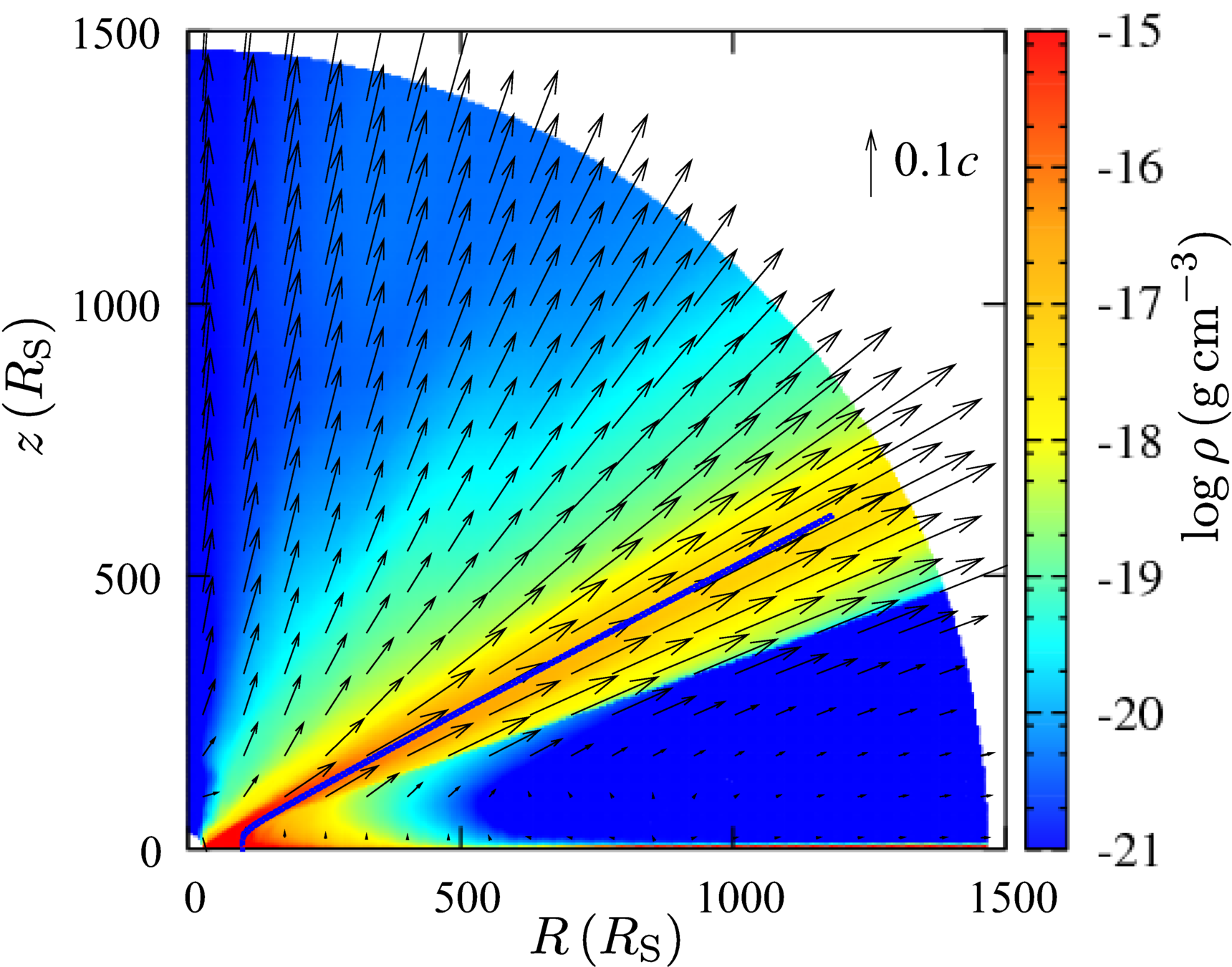
Disc radius [Rs]
Height [Rs]
Density
Nomura et al (2018)
Hydro
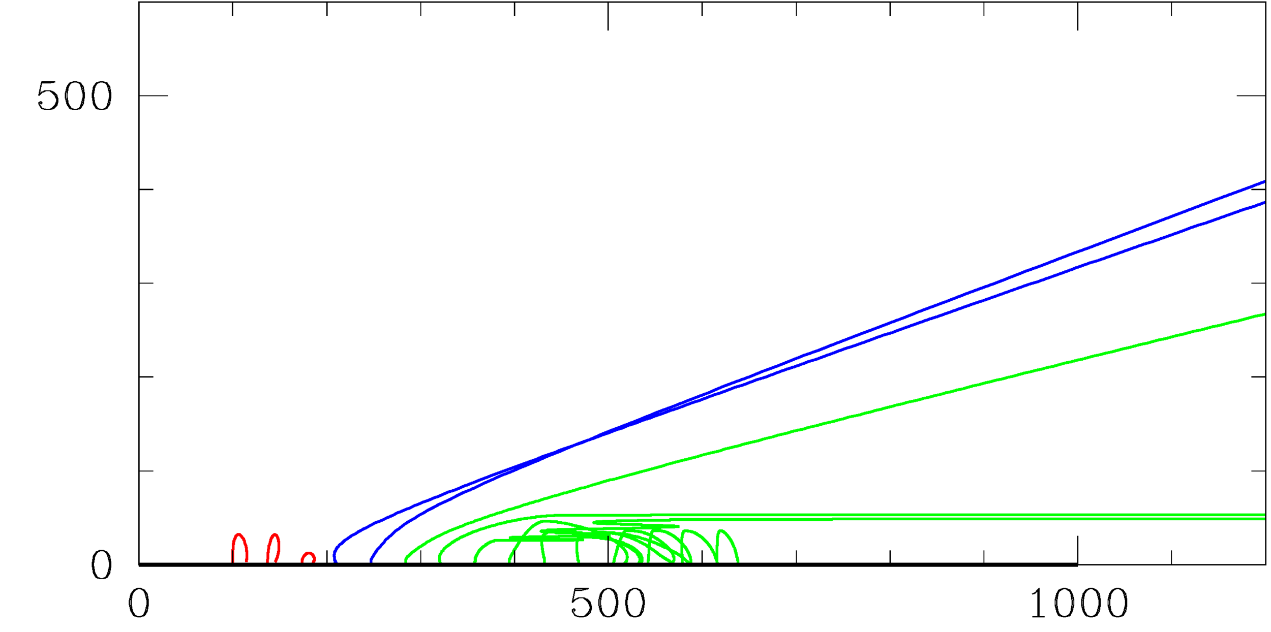
Disc radius [Rs]
Height [Rs]
Qwind model, Risaliti & Elvis (2010)
Non-hydro
- Accounts for gas pressure and heating/cooling.
- Slow
- Neglects gas pressure forces.
- Lots of independent input parameters
- Very fast.
Shielding
Our goal: improve Qwind (non-hydro)
Following the same non-hydro approach, we are working on a new code with major improvements:
- Fully written in Python while keeping performance, and open source.
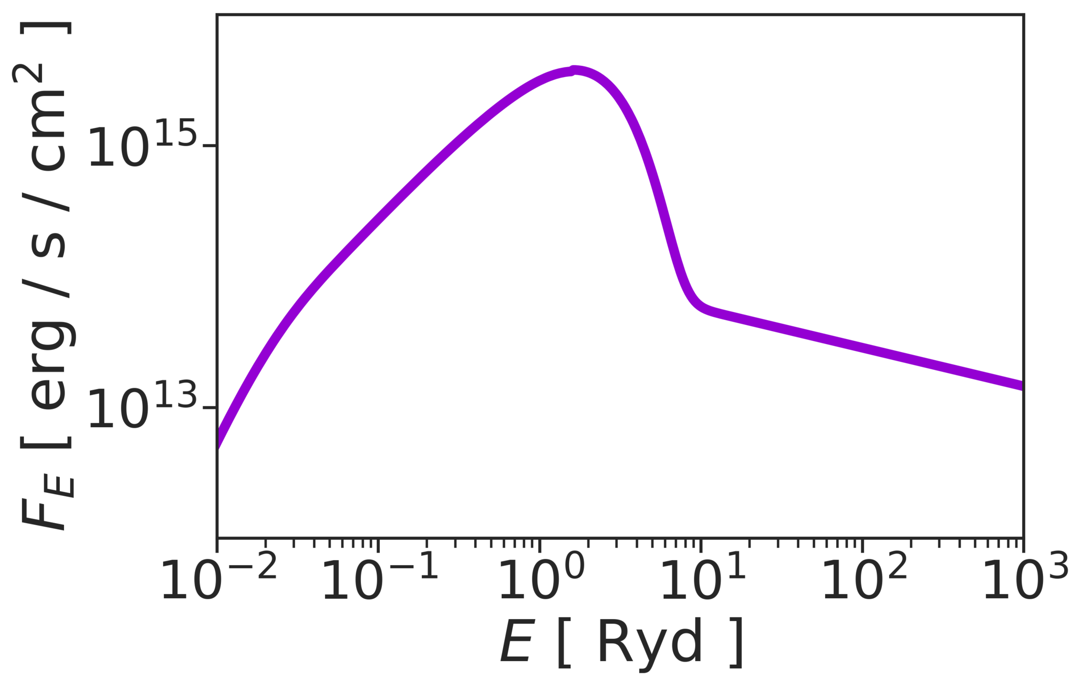
- Sensitive treatment of the radiation field, motivated by Cloudy runs.
- Reduced number of input parameters.
- Self-consistent with the disc structure, i.e, mass loss due to wind should change accretion rate, and thus luminosity.
X-Ray opacities with Cloudy
Current simulations overestimate X-Ray obscuration.
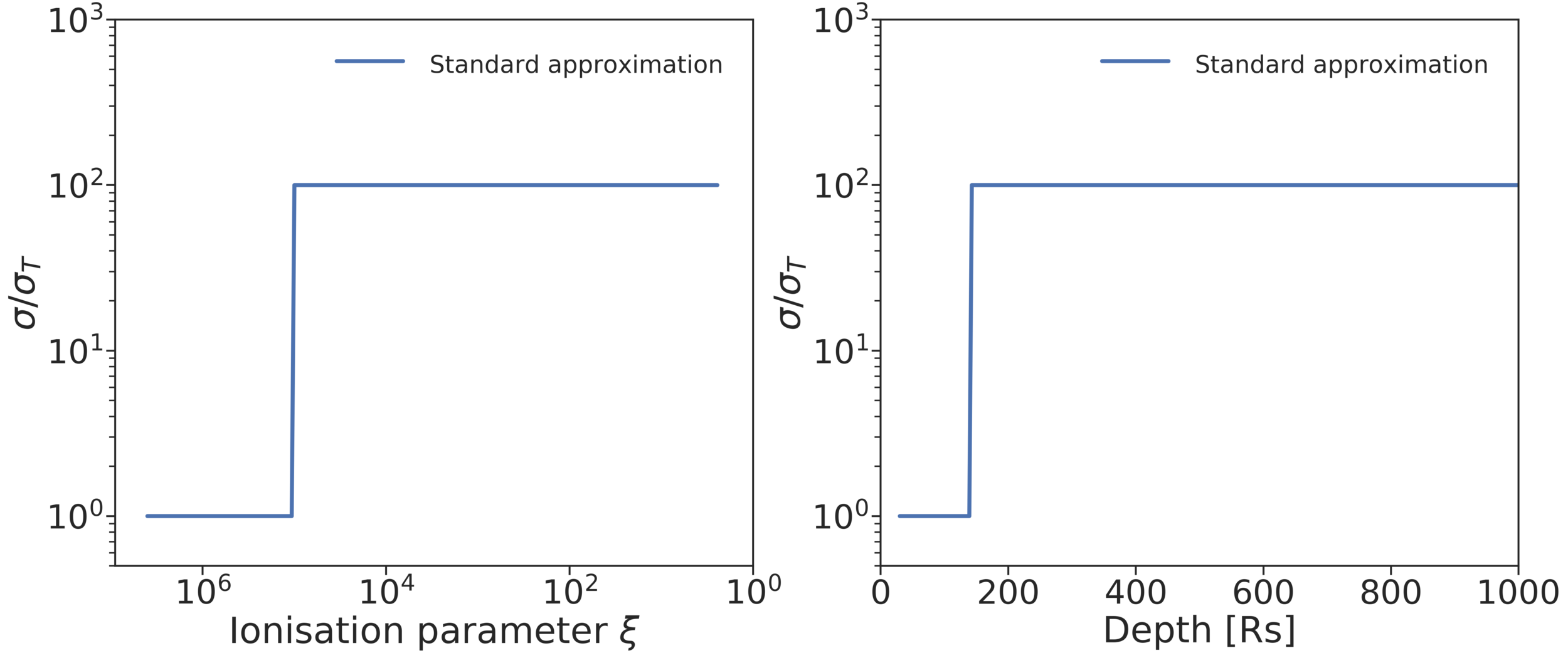
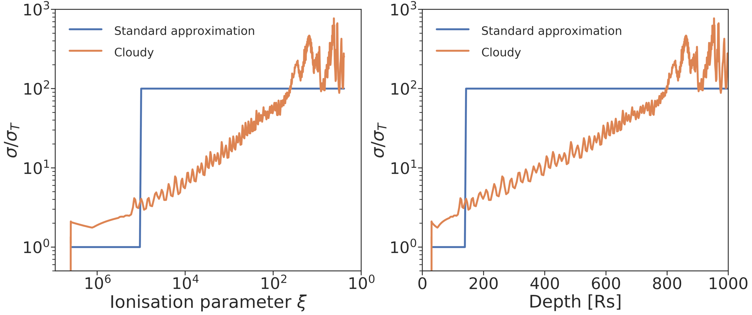
\sigma_\text{X} = \begin{cases}
\sigma_\text{e.s.} & \text{ if } \xi > 10^5 \\
100\sigma_\text{e.s.} & \text{ if } \xi < 10^5
\end{cases}
How bad is it?
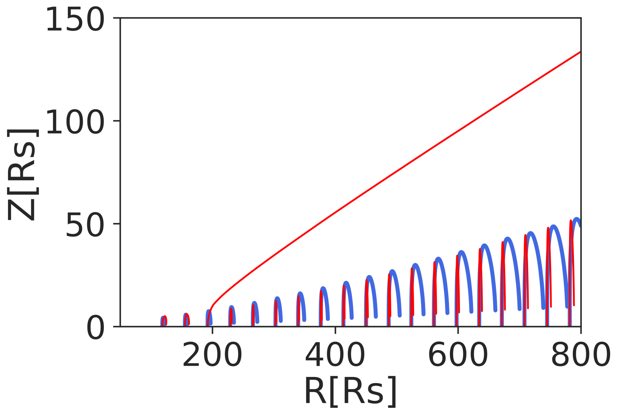
Qwind code, old Opacities
New opacities,
with no UV obscuration
Conclusions
- AGN Feedback is one of the cornerstones of cosmological simulations.
- Line-driven winds are a strong candidate for setting M-σ relationship, as well as the feedback efficiency.
- We need to improve our line-driven winds models, making them more physically motivated and self consistent.
TO-DO
- Improve numerical code for line-driven winds.
- Scan parameter range to deduce feedback efficiency.
- Implement new feedback scheme in cosmological simulations.
Simulating AGN feedback
By arnauqb


