Calibrating large-scale ABMs
Arnau Quera-Bofarull
A case study: the JUNE epidemiological model
June Dalziel Almeida
The JUNE
agent-based model
github.com/IDAS-Durham/JUNE
Many other epi ABMs exist:
- Covid-sim
- Covasim
- OpenABM
- etc.
What makes JUNE special?
England digital twin
England Digital twin
Geography

England Digital twin
Demography
- age (27)
- sex (f)
- ethnic group (Caribbean)
- deprivation index 2 (1-10)
- work sector / subsector (healthcare/doctor)
- mode of transport (public)
- area of residence
- super area of work

Main data source: census data (NOMIS)
~56 million agents
male
female
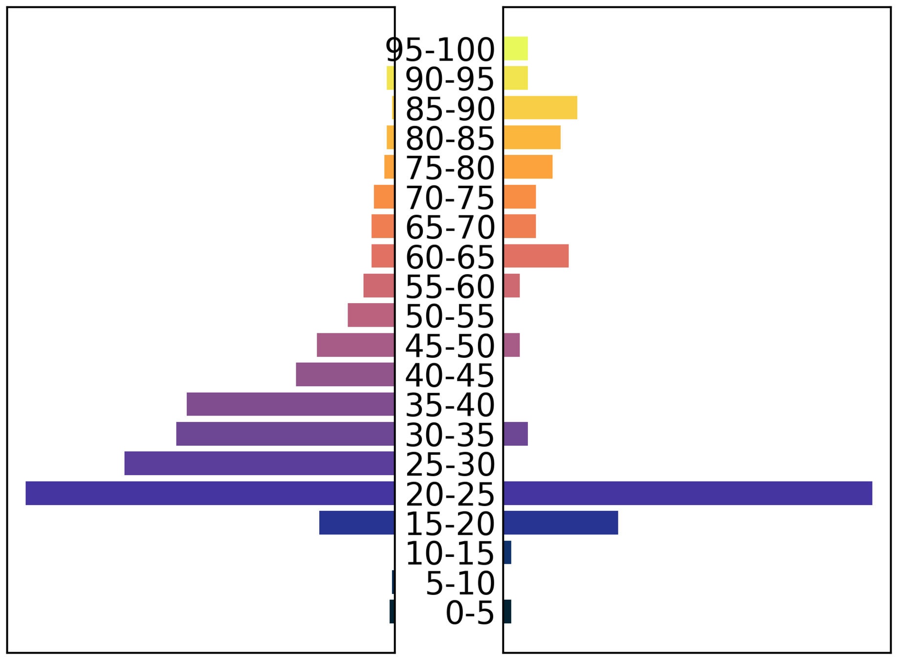
Demographic granularity
male
female
England Digital twin
Dynamics (where can people go?)
- Residence
- Care Home
- Household
- Primary activity
- Company
- Hospital
- School
- Care Home
- University
-
Travel
- Commute
- National travel
- Leisure
- Shopping
- Pubs / restaurants
- Cinema
- Gyms
- Residence visits
City of London workers' usual residence
Matching workplace and residence
Commute
-
Census -> method of transportation.
-
Two kinds: Inner city commute, outer city commute


Hub

Hub
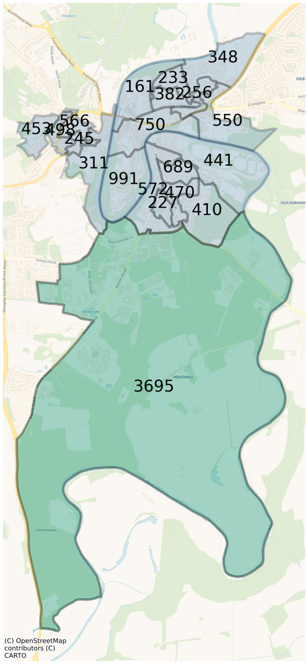
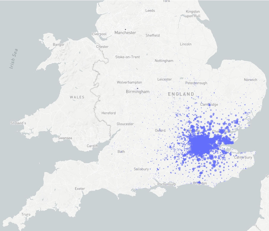
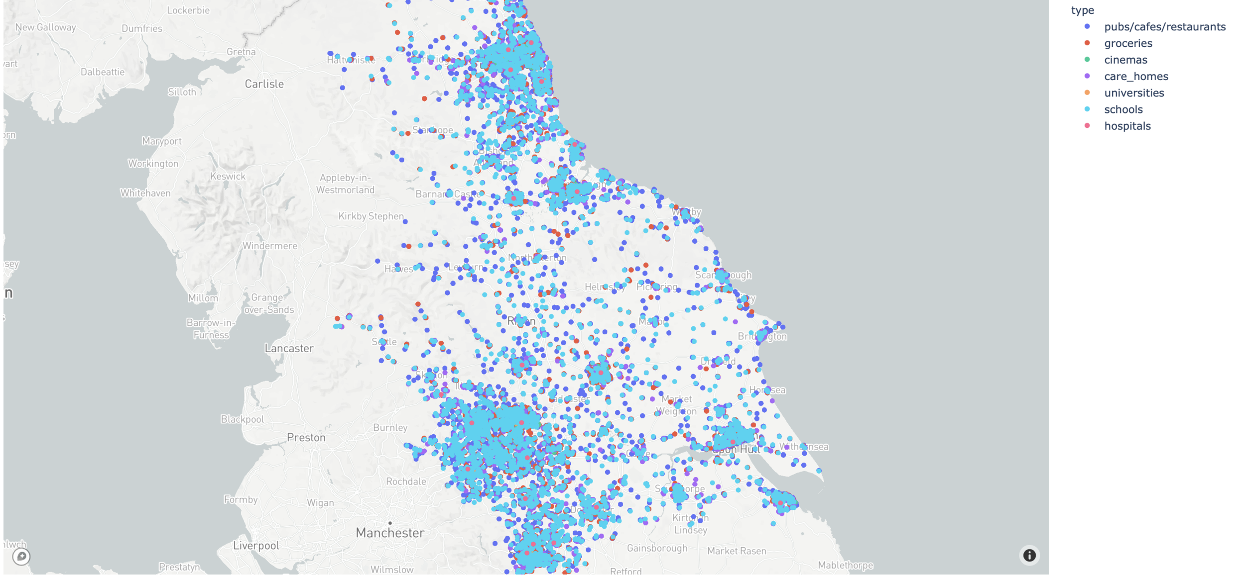
Venues geolocalisation

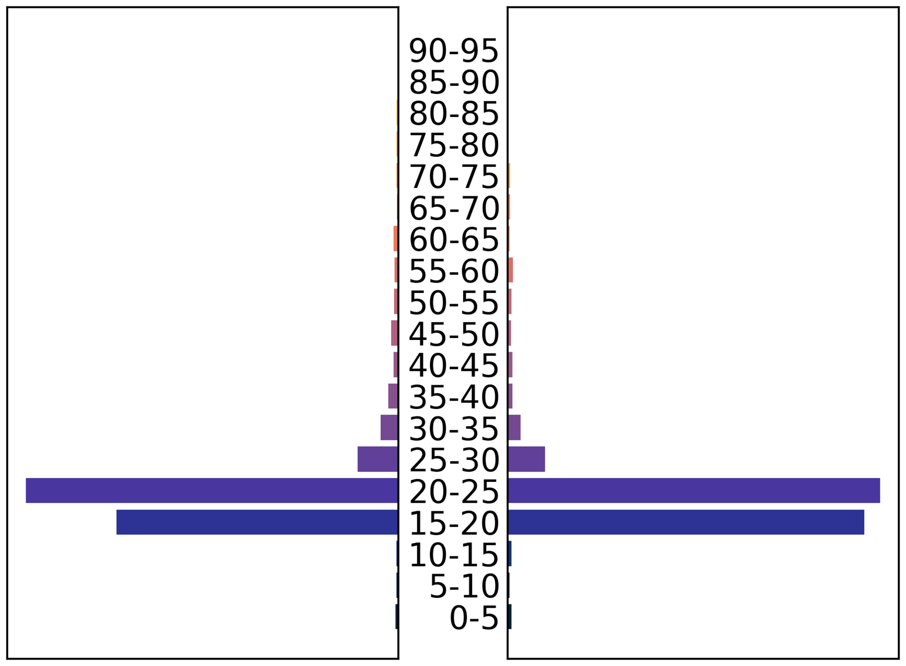
Durham student population

43 yo
38 yo
10 yo
Infection transmission
j
j
i


Intensity of contacts (per group)
Infectiousness profile

Contact
Matrix
p_i = 1- \exp\left({-\lambda_{ij}\;\Delta t}\right)

Disease Trajectory
Odds calibrated to data
import scipy
Policies

The challenge of calibration
Very detailed model, but
is it useful?
is it realistic?
can we 'fit' it?
The challenge of calibration
Unknown parameters:
-
Location contact intensity (13)
-
Effectiveness of policies (5)
-
Seed cases (1)
19 parameters to fit
JUNE's computational cost
typical England run ~ 600 CPU hours / 100 GB RAM

Parallelisation by domains of equal population
Very expensive!
History matching and Bayesian emulation
Train Bayesian emulator
Run emulator
O(500k) times
Run full simulation O(100) times
Discard implausible regions
Sample O(100) parameter sets from latin hypercube
Sample O(100) parameter sets from non-implausible region

History matching in JUNE
Why we needed the complexity
JUNE reproduces infection disparities among various demographic groups thanks to its granularity.

Current work
ABMs as Graph Neural Networks
Idea:
Represent the ABM as a graph and code it using a GNN library (like PyTorch)
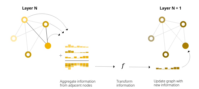
What is a Graph Neural Network?
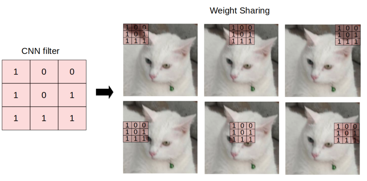

\mathbf{m}_{j\to i} = \phi(\mathbf{x}_i, \mathbf{x}_j, \mathbf{e}_{j\to i})
Message Passing
\bar{\mathbf{m}}_{i} = \square_{j\in N(i)} \mathbf{m}_{j\to i}
\mathbf{x}_{i}' = \gamma_x(\mathbf{x}_{i}, \bar{\mathbf{m}}_{i})
\mathbf{e}_{j\to i}^\prime = \gamma_e(\mathbf{e}_{j \to i},\mathbf{m}_{j \to i})
Node
Edge
Message
Convolution
"Average" Message
Updated node
Updated edge
Convolution
Update node function
Update edge function
Representing JUNE as a (heterogeneous) graph
i_1
i_2
i_3
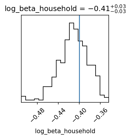
I = \beta_\mathrm{household} \times \sum_j i_j
I \times s_1
I \times s_2
I \times s_3
I
I
I
Representing JUNE as a (heterogeneous) graph
t_2
t_1
t_1
t_3
Implementation in PyTorch
Advantages:
- Runs on GPU: Massive performance boost.
JUNE
O(100) CPU hours
Torch JUNE
O(10) CPU seconds
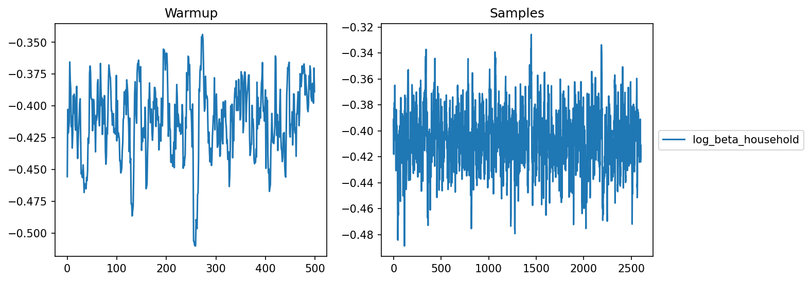
Implementation in PyTorch
2. Automatic differentiation
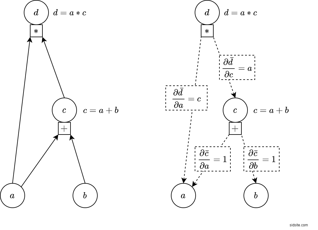
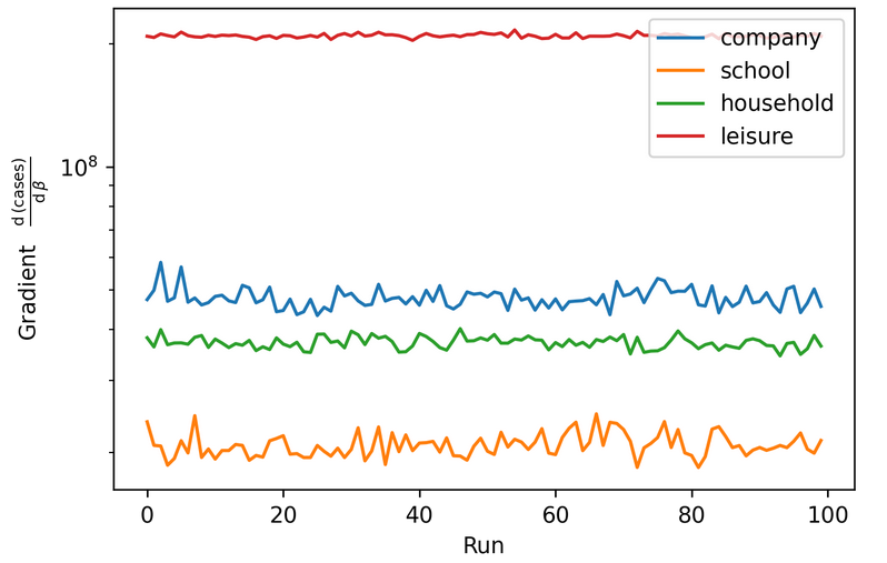
Differentiation enables gradient assisted inference (like HMC)
Backup slides
Bayesian emulation
\text{Model: }\;\;(x_1, \dots, x_d) \to (f_1(x), \dots, f_q(x))
contact intensity in pubs
hospitalisations
f_i(x) = \text{Gaussian process}(x_A) + \text{Noise}(x)
Emulation:
Bayesian emulation
The emulator returns
\mathrm{E}[f_i(x)]
\mathrm{Var}(f_i(x))
on new unexplored points, but several orders of magnitude faster than the original model
Training the emulator
- Run the simulator on n points
D_i = (f_i(x^{(1)}), \dots, f_i(x^{(n)}))
and obtain:
2. Update the emulator's paramaters using Bayes linear methods

Linking the model to reality
-
Observational
-
Model discrepancy
z = y + e
y = f(x^*) + \epsilon
History matching
Goal: Find all sets of input parameters that lead to acceptable matches.
Method: Iteratively rule out implausible parameter sets.

Reject when
I > 3

Visualising the non-implausible regions
Complexity group update
By arnauqb


