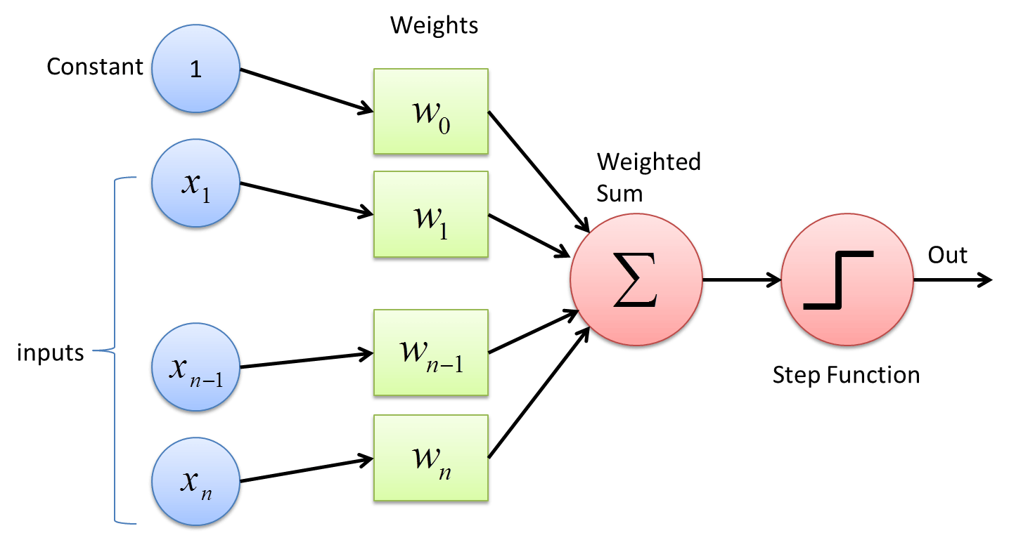
Perceptron / Neuron
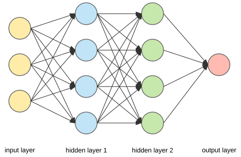
Neural Network
Goal: optimise some loss function (mean square error, cross-entropy...)
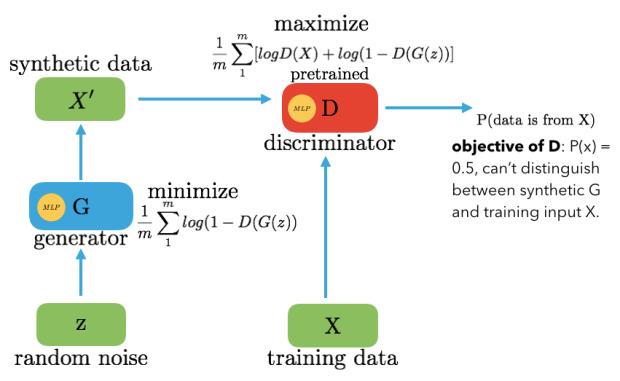
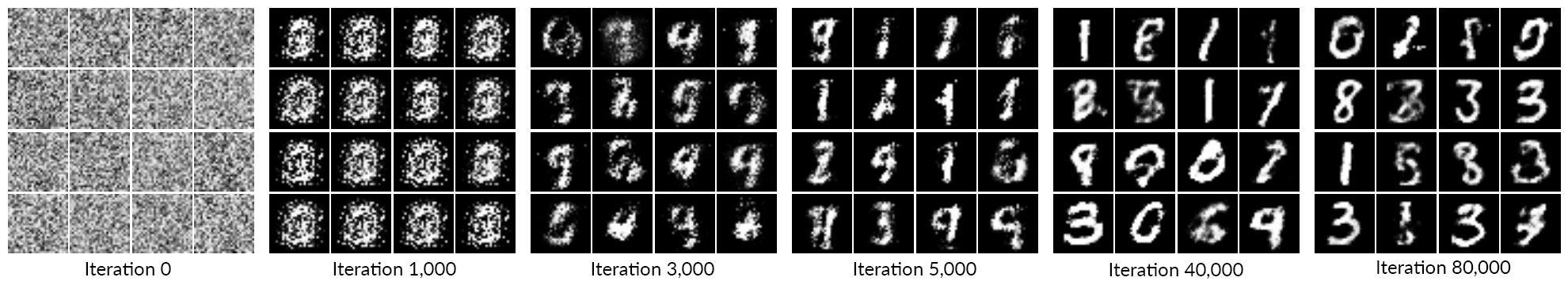
Generative Adversarial Network (GAN)
We want to:
- Learn the distribution that generates the data p(x).
- Generate new samples from p(x)
How we do it:
- Two CNNs: Generator G and Discriminator D.
- We train G to generate new "fake" samples to trick D.
- We train D to distinguish fake and real samples.
- Training ends when there is a "stalemate".
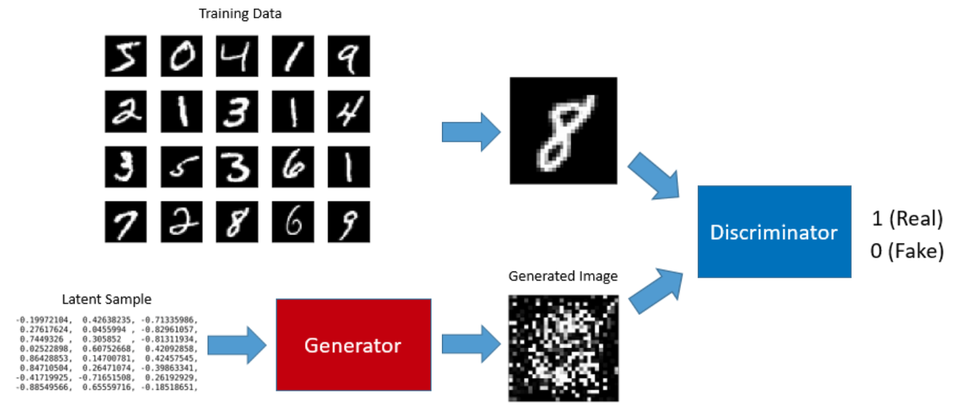
Generative Adversarial Network (GAN)
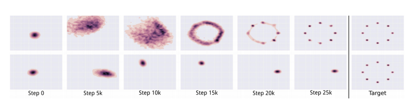
Example
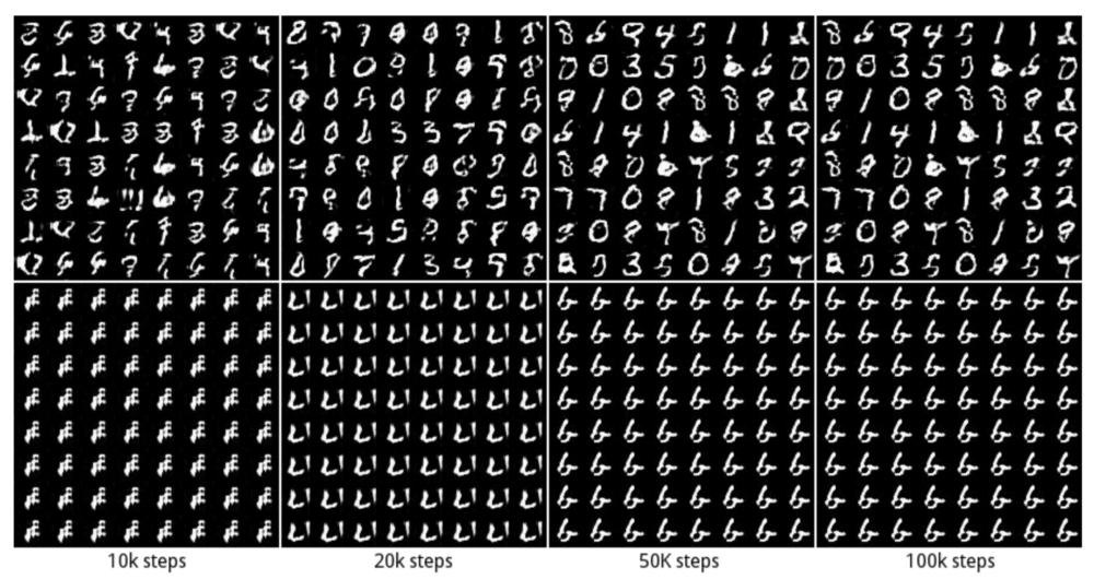
GANs are hard to train.
Mode collapse
The generator may not generate samples from the whole distribution,
which means the optimiser got stuck at a local minimum of the generator loss function.
The GAN loss function
minimax game:

The training stops when "Nash equilibrium" is reached, but what is that?
Consider the following game:
Player A chooses one number and player B another one, the goal of player A is to minimize the product of the two, and the goal of B is to maximise it.

The Nash equilibrium is reached when one player does not change his/her strategy regardless of what the other player does.
So, for which values of x (or y) is the Nash equilbrium reached?
x=y=0
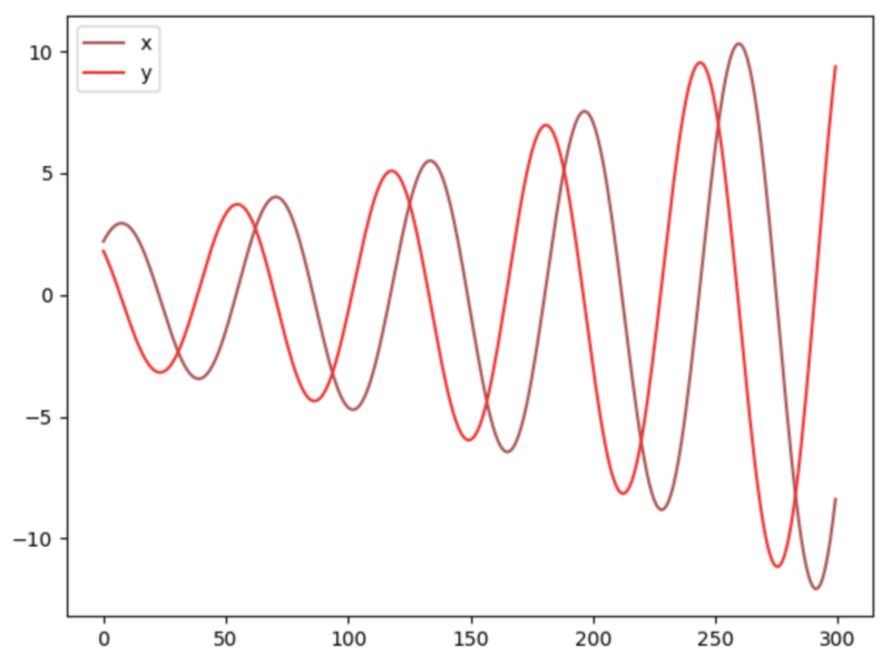
Conclusion: cost functions might not converge using gradient descent in a minimax game.
Where does the GAN loss function (or any other in general) come from?
Machine Learning: an information theory approach.
Credit: Marc Sastre
How is the weather in Durham?
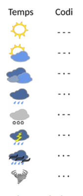
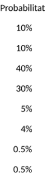
Idea: events contain a certain amount of measurable information.
I(x) = - \log(\,p(x)\,)
Rare events "carry" more information.
Main reference:
https://medium.com/@jonathan_hui/gan-why-it-is-so-hard-to-train-generative-advisory-networks-819a86b3750b
Entropy
H(x) = E_{x\sim p} \left[\, I(x) \,\right]
= - \sum_x p(x) \log(p(x))
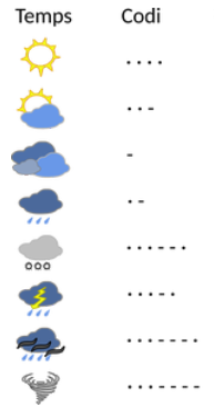
If we take the logarithm to have base 2, then the entropy can be interpreted as the minimum number of bits required to encode the information.
Example: coin
H(x) = -p(\text{head}) \log_2 p(\text{head}) - p(\text{tails})\log_2p(\text{tails})
= -\log_2 \frac{1}{2} = 1
Example: dice
H(x) = \dots = 2.59
Cross-entropy
H(p,q) = E_{x \sim p} [ q(x) ]
= - \sum_x p(x) \log(q(x))
Measures the minimum number of bits to encode an event x, generated from p using the optimal scheme for q.
Machine Learning ( or Bayesian statistics in general)
- Data points generated from p.
- We want to find q that is "as close as possible to p".
"Distance" between two probability distributions: KL divergence.
D_{KL} ( p || q) = E_{x \sim p} \,\log\left( \,\frac{p(x)}{q(x)}\,\right)
Not commutative! (so not a proper distance...)
Expanding it...
D_{KL} (p||q) = \underbrace{\sum_{x=1}^N p(x)\log p(x)}_{-H(p)} - \underbrace{\sum_{x=1}^N p(x)\log q(x)}_{-H(p,q)}
\text{So, } H(p,q) = H(p) + D_{KL} (p || q)
If p is fixed, then minimising the cross-entropy is equivalent to minimising the KL divergence.
Fun fact
Since D_KL is always positive, p=q is a minimum ( as we would expect).
Expanding around this minimum we get:
D_{KL}(p||q) \approx \frac{1}{2} \, \delta \theta^j \, \delta \theta^i \, g_{ij}( \theta_0 )
The Hessian of D is the Fisher information matrix. Gives the "informational difference" between two close points on the "parameter hyperspace".
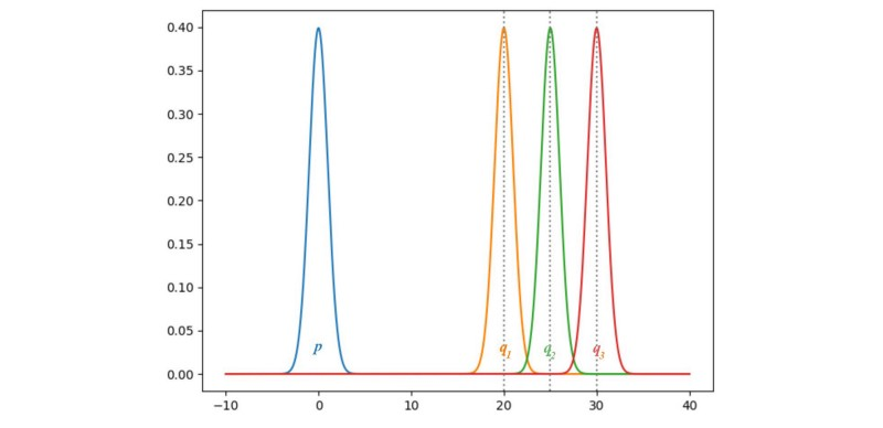
Why is D_KL not commutative?
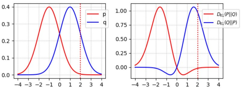
- D(p||q) penalises low image variety.
- D(q||p) penalises low quality.
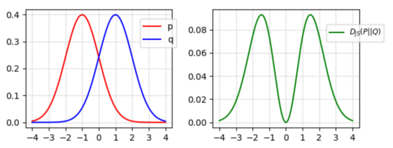
GANs try to balance this. If we symmetrise D_KL:
D_{JS} (p || q) = \frac{1}{2} D_{KL} \left( p || \frac{p+q}{2} \right) + \frac{1}{2} D_{KL} \left(q||\frac{p+q}{2}\right)
If we assume a perfect discriminator, the GAN loss function reduces to:

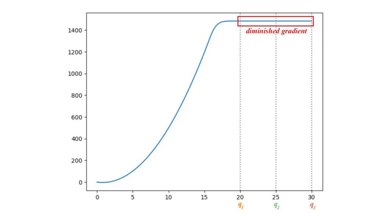
People try different cost function to avoid the vanishing gradient problem.
Why mode collapse?
Extensively studied, still not very well understood.
Training set
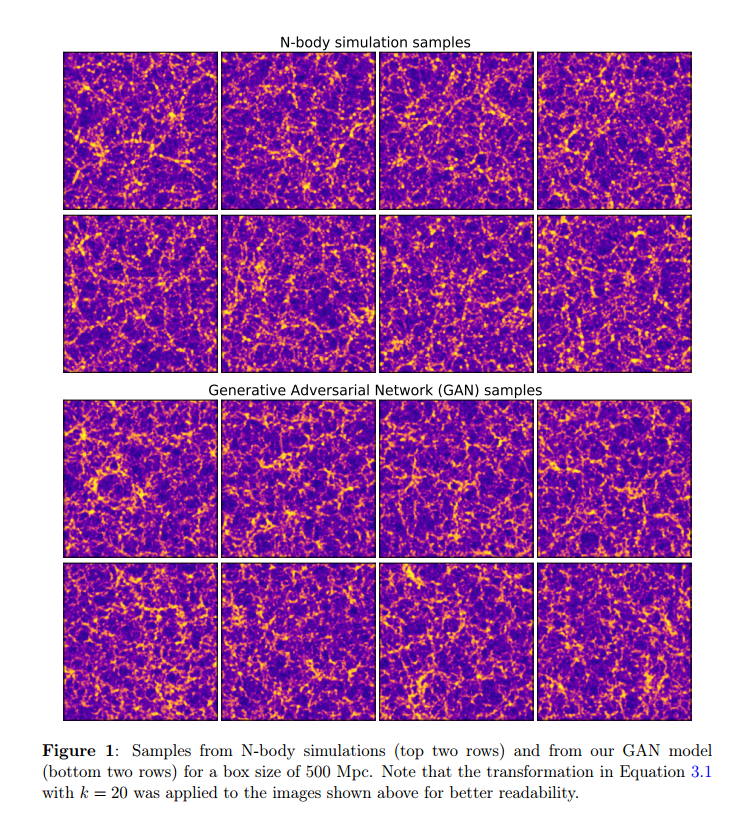
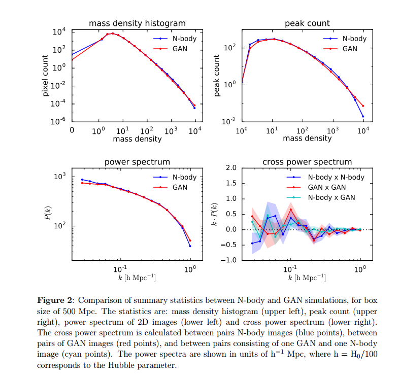
Results for box size of 500 Mpc.
Results for box size of 100 Mpc.
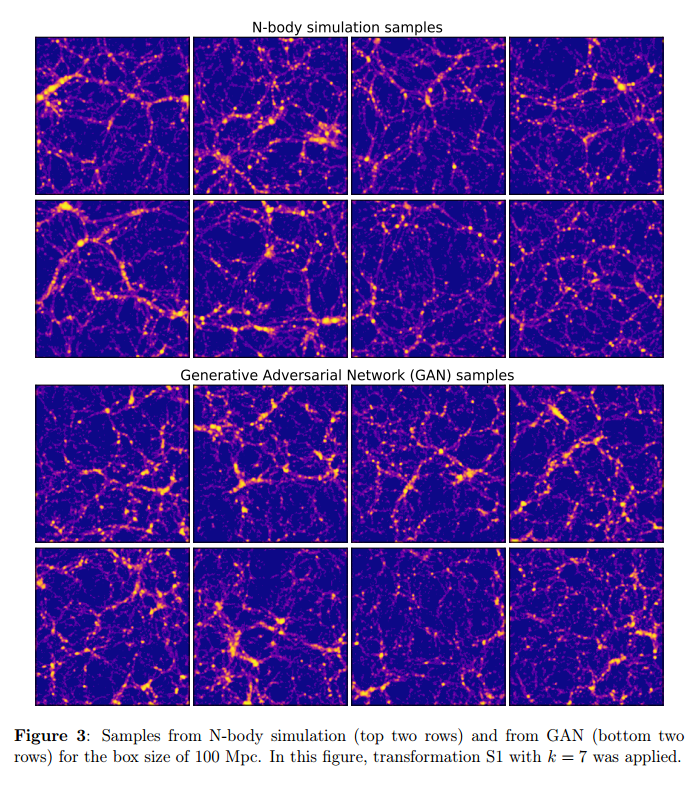
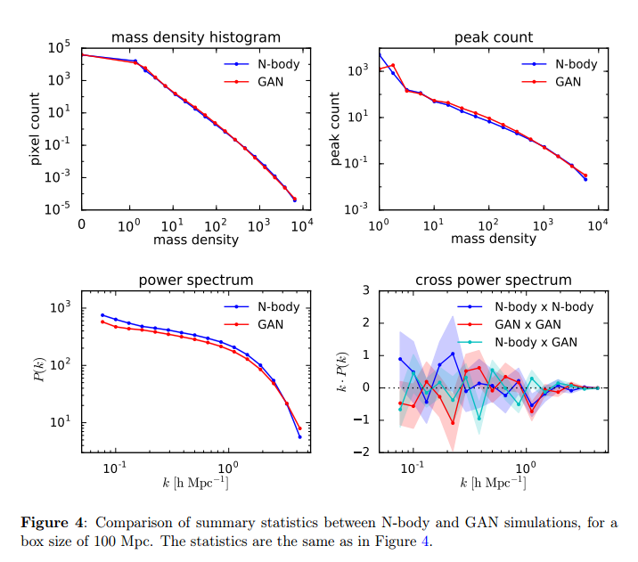
Fast Cosmic Web Simulations with GANs
By arnauqb


