Qwind
Simulating UV line-driven winds in AGNs
Arnau Quera-Bofarull
Supervised by:
Ken Ohsuga - Tsukuba University
Cedric Lacey, Chris Done - Durham University
What is AGN feedback?
Energy coupling between the central black hole and its host galaxy.
\frac{\text{size of BH}}{\text{size of Galaxy}} \approx

Joint evolution of BH and host Galaxy
Black Hole Mass
Bulge velocity dispersion

Kormendy & Ho (2013)
Effects on galaxy population.
Image credit: Mutch et al (2013)
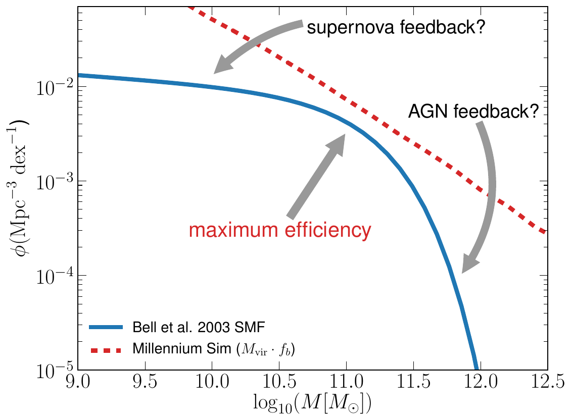
Mass
Mass Function
(log) Mass Number Count
Stellar Mass
Schaye et al (2014)
AGN (and supernova) feedback are needed to match observations.
The origin of the coupling: Accretion
E = \eta m c^2
\text{ BH accretion } \rightarrow \eta \approx 0.1
Credit: NASA/Goddard Space Flight Center
- Matter falls in gaining kinetic energy.
- Part of this energy released as radiation.
Fun fact: throwing 300kg down to a black hole powers all Japan for a year!
Is that enough to alter the galaxy?
E_\text{outflow} \approx 0.1 M_{BH} c^2 \approx 10^{61} \text{ erg}
\text{Consider a BH grown through accretion to } M = 10^8 M_\odot
\text{Consider a galaxy bulge with } M=10^{11} M_\odot \text{ and } \sigma_v = 200 \text{km}/\text{s}
E_\text{binding} \approx M_\text{bulge} \sigma_v^2 \approx 10^{58} \text{ erg}
More than enough energy...
Can this radiation be (minimally) coupled with the surrounding material?
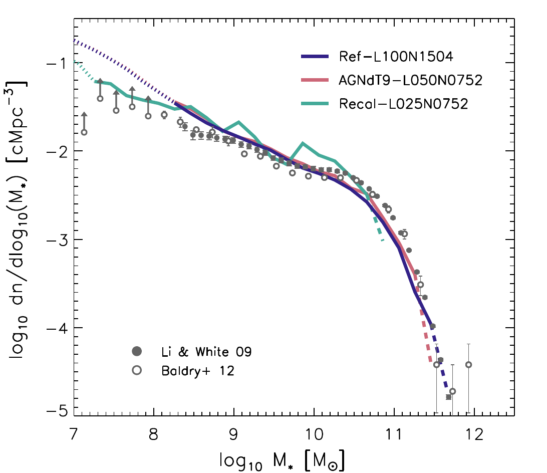
Eagle AGN feedback
In EAGLE, a fraction of the radiated energy from accretion is coupled thermally to the surrounding gas.
\dot E_\text{inj} = \epsilon_f \dot E_\text{acc.}
Calibrated to match observations (ϵ = 0.15).
Since final BH masses depend on it, they are not a prediction of the simulation.
Ideally, ϵ should be derived from first principles.
\epsilon_f = \epsilon_f ( M_\text{BH}, \dot M, a)
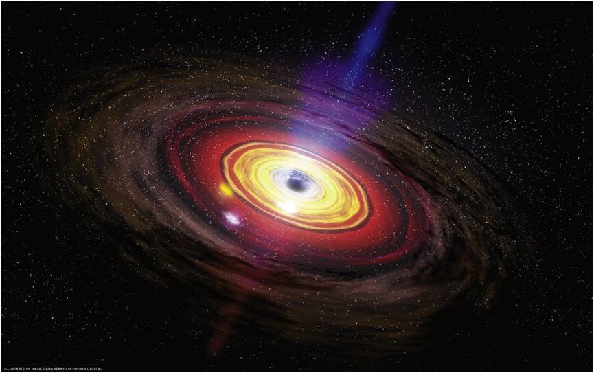
Feedback mechanisms
Radiative mode
Kinetic mode
Winds
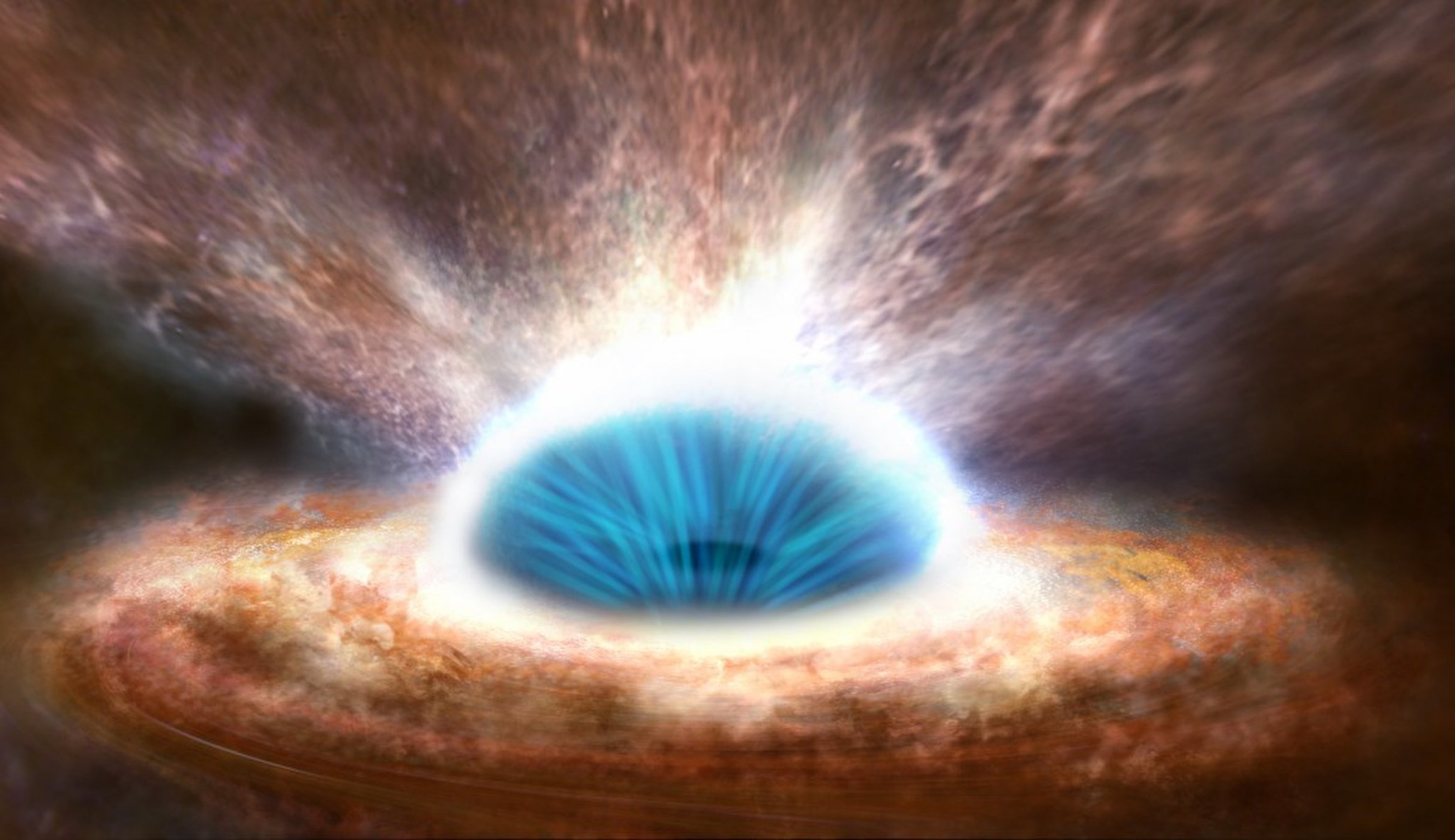
Credit: ESA/ATG medialab
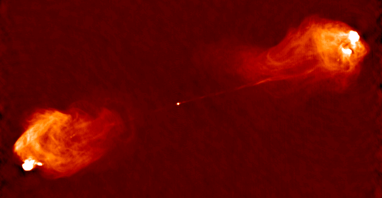
Credit: NRAO/AUI
Jets
Radiation vs Gravity
The Eddington Limit
g_\text{rad} = g_\text{rad}\left( \kappa , L\right)
Luminosity
Opacity
g_\text{grav} = g_\text{grav}\left(M_\text{BH}\right)
\text{Assuming } \kappa = \kappa_{e.s.} \text{, both quantities are equal at }
L_\text{Edd} = \frac{4 \pi G M_\text{BH} c}{\kappa_\text{es}}
How do we create a wind?
L>L_\text{Edd} \longrightarrow \text{ Super Eddington winds}
\kappa > \kappa_\text{e.s.} \longrightarrow \text{Line-driven winds}
Radiation vs Gravity
The line-driving mechanism
Opacities can be much larger than free electron scattering.
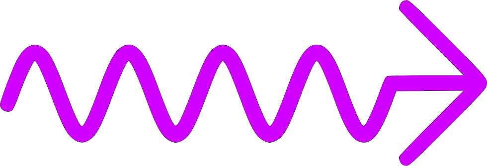
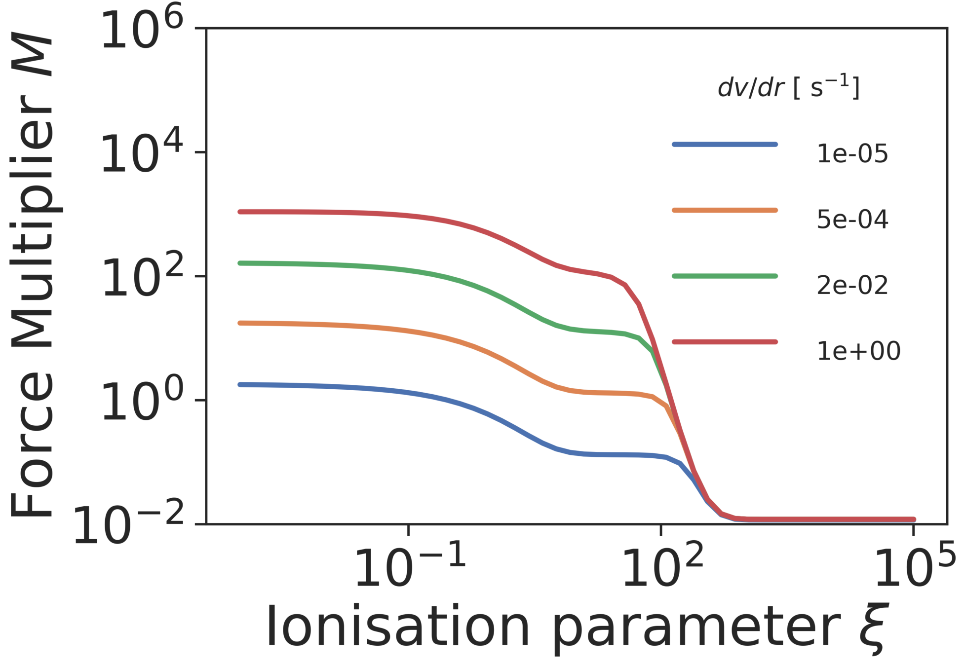
\frac{\kappa_\text{lines + e.s.}}{\kappa_\text{e.s}} = M\left( \frac{dv}{dr}, \xi \right)
v
\xi \propto L_\text{X-Rays}
Ionisation parameter
Castor, Abbot & Klein (1975)
Force Multiplier
X-Rays vs UV
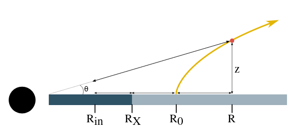
The setup
Need to shield against X-Rays
Simulating line-driven winds
Different approaches
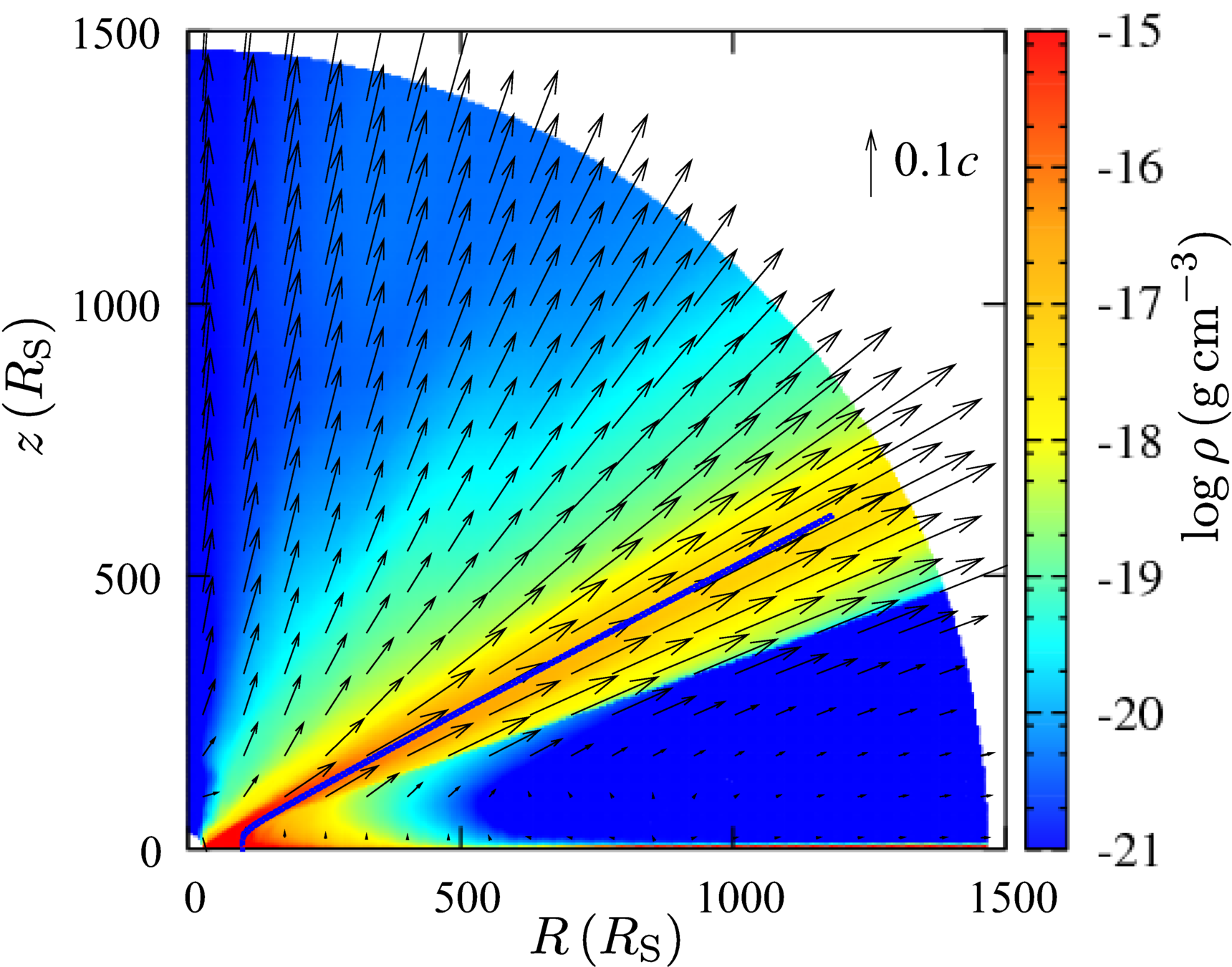
Disc radius [Rs]
Height [Rs]
Density
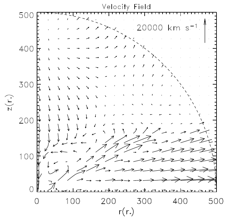
Nomura et al (2018)
Hydro
Disc radius [Rs]
Height [Rs]
Qwind model, Risaliti & Elvis (2010)
Non-hydro
- Accounts for gas pressure and heating/cooling.
- Slow
- Neglects gas pressure forces.
- Lots of independent input parameters
- Very fast.
Shielding
Revisiting Qwind
Key general assumptions
- Wind modeled as a set of streamlines
- Gas parcels are launched from the disc, and evolved according to their equation of motion
- Gas pressure is neglected (supersonic wind)
Revisiting Qwind
Radiation treatment assumptions
- Simple X-Ray opacity law
- Optical depths are calculated from the center of the grid
\sigma_X = \begin{cases}
100\sigma_T & \mathrm{ if } &\xi &< 10^5\\
\sigma_T & \mathrm{ if } &\xi &\geq 10^5
\end{cases}
Revisiting Qwind
- Code release with significant techincal improvements
(Quera-Bofarull et al. (2020)): arXiv:2001.04720
github.com/arnauqb/qwind
"Qwind 1"
"Qwind 2"
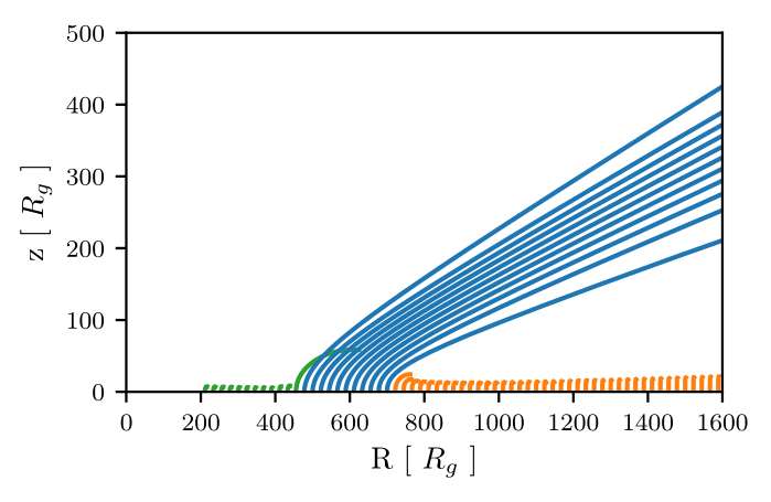
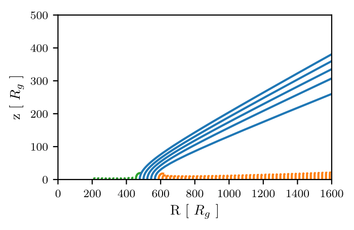
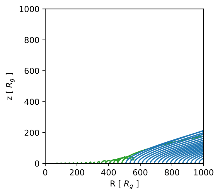
A case study
M=10^8\; M_\odot \;,\; \dot m = 0.5
- Free input parameters:
- T
- Example
\dot M_\mathrm{wind} = 8 \times 10^{-3} M_\odot / \mathrm{yr} \approx 0.4 \% \,\dot M \\
L_\mathrm{kin} \approx 0.03 \% L_\text{Eddington}
Too low for feedback...
n_0, \, v_0, \, z_0
n_0 = 2 \times 10^8\; \text{ cm}^{-3} \\
v_0 = 10^7\; \text{ cm s}^{-1} \\
z_0 = 1 \;R_g \\
T = 2.5 \times 10^4 \; \text{K}
A case study
M=10^8\; M_\odot \;,\; \dot m = 0.5
... but Qwind strongly depends on the initial density and velocity of the streamlines
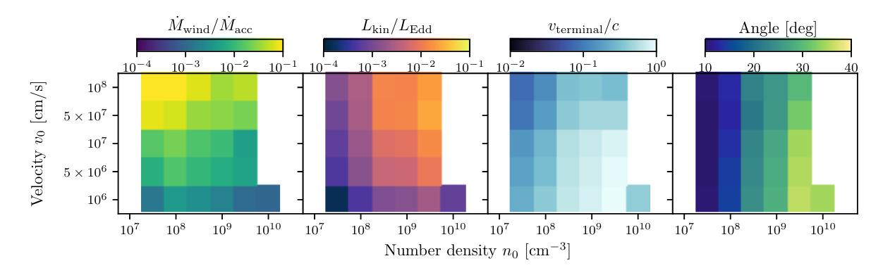
Need physical model for initial conditions
TO DO LIST
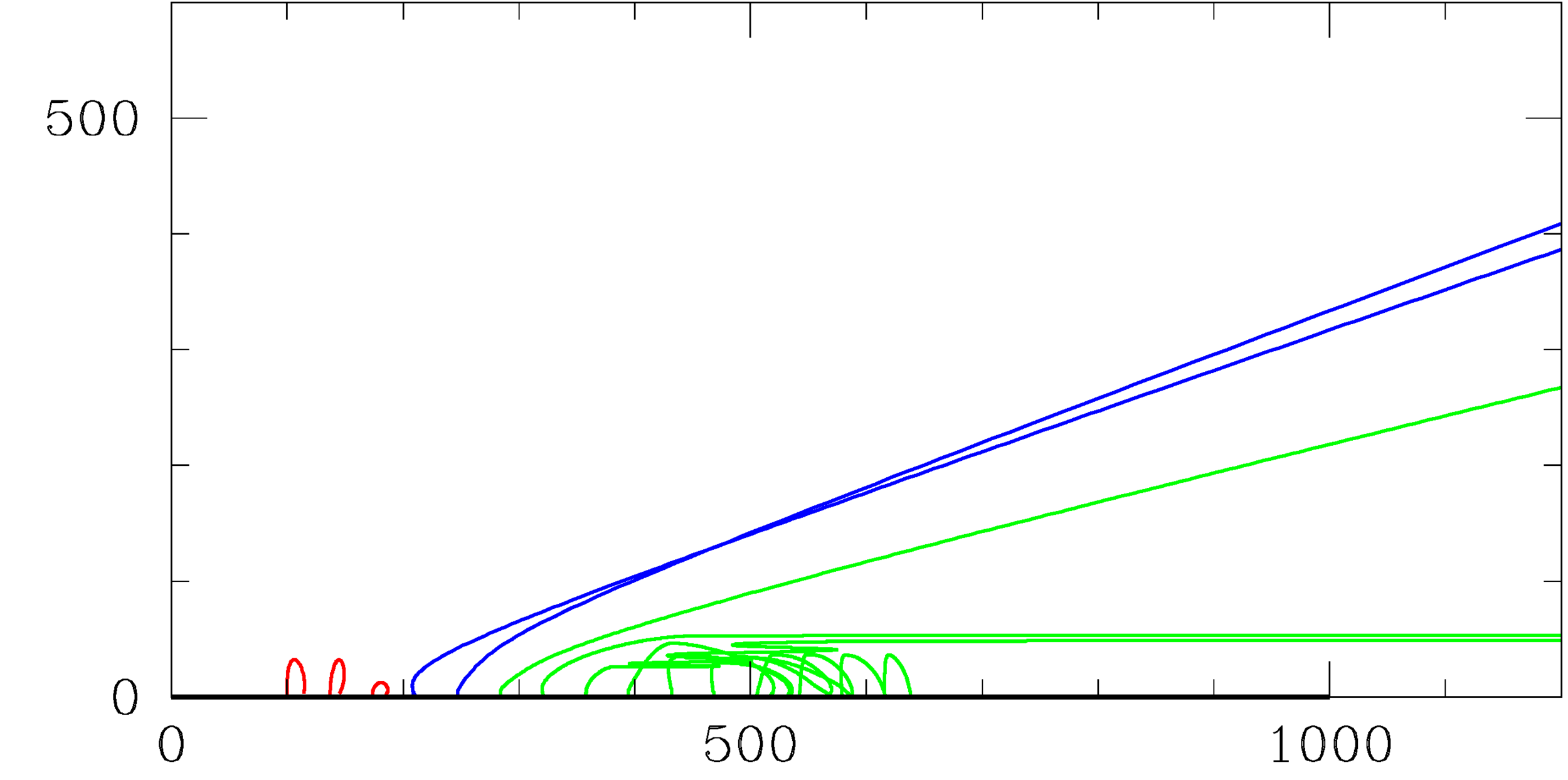
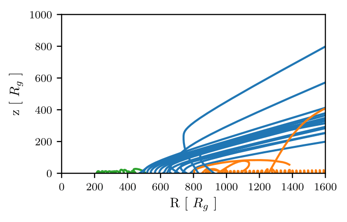
A case study, comparison with hydro
M=10^8\; M_\odot \;,\; \dot m = 0.5
- We can compare the results our model with a hydrodynamic simulation (Proga et al 2004), setting the same parameter values.
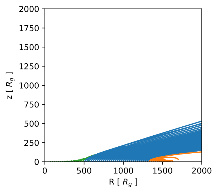
\text{Qwind}\\
\dot{M}_\text{wind} = 0.3 \; \text{M}_\odot / \text{yr} \\
v_\text{terminal} \in (0.016-0.18) c
\text{P04}\\
\dot{M}_\text{wind} \in (0.16 - 0.3) \; \text{M}_\odot / \text{yr} \\
v_\text{terminal} \in (0.006-0.06) c
Future work
Text
- We are currently improving the Phyiscs of Qwind
Realistic optical depths...
... with physically motivated SEDs
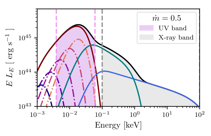
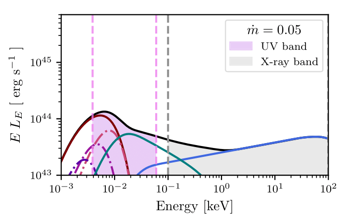
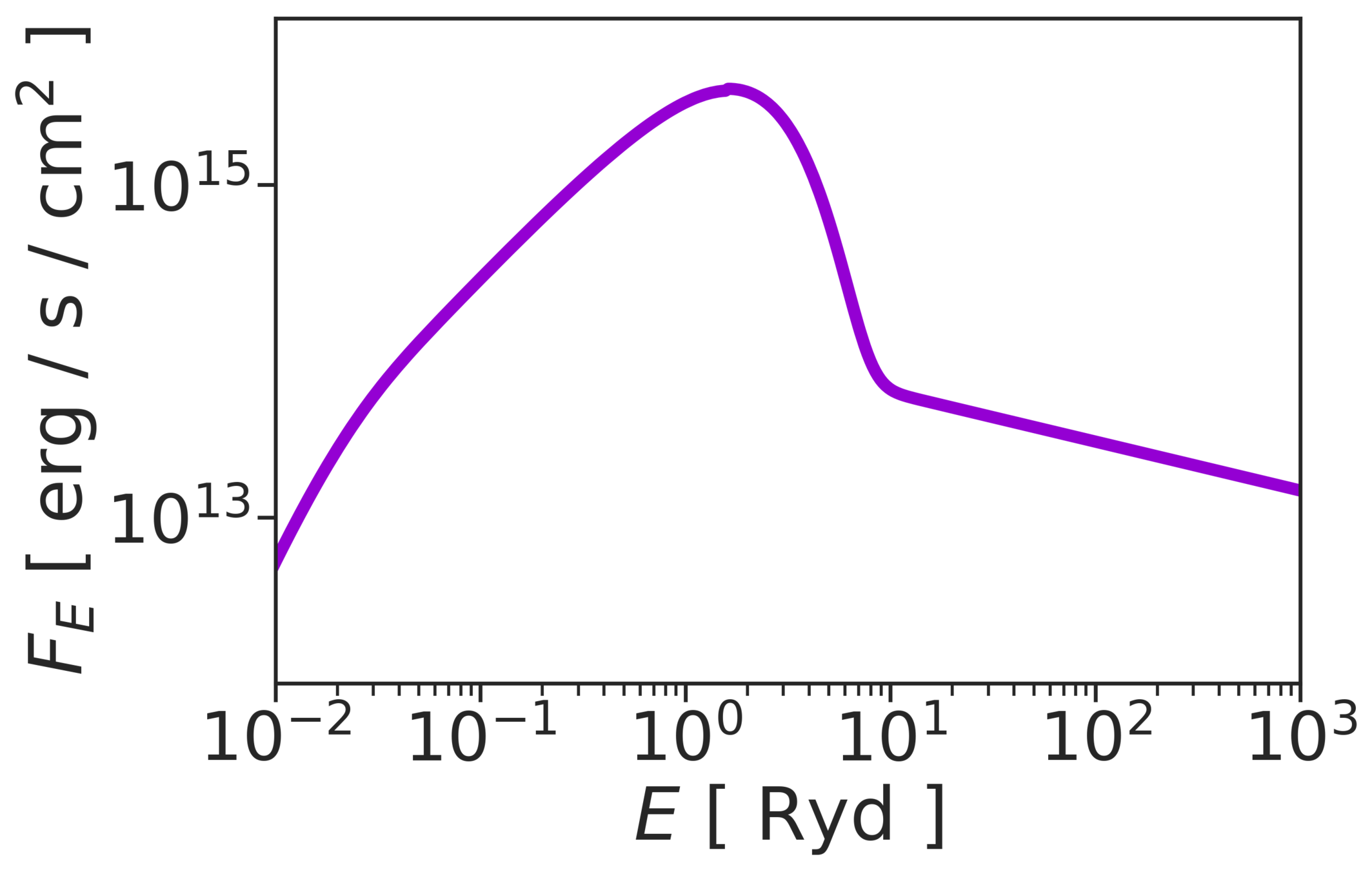
\dot m = 0.05
\dot m = 0.5
Kubota & Done (2016)
Future work
Text
Self-consistent accretion rate
\dot M
\dot M_\text{wind}

We can easily identify where the wind is coming from, and subtract it to the local accretion rate
Future work
Text
Physically motivated initial conditions
- Model disc annuli as O-stars (Nomura 2012)
- Use 1D analytical solution locally at the disc surface
- Use 1D analytical solution locally at the disc surface
- Another option: "Solve" vertical disc structure.
Stay tuned for updates!
Conclusions
Text
- Subgrid models of AGN feedback in cosmological simulations need to be more physically motivated.
- Qwind model able to mimic results of hydrodynamic simulations at a much lower cost.
- Realistic radiation transfer and physical initial conditions, most important improvements to do.
Thank you! Questions?
Quera-Bofarull et al. (2020) : arXiv:2001.04720
Try the code at github.com/arnauqb/qwind
Qwind Hokkaido
By arnauqb


