UV line-driven winds:
Dependence on black hole Properties
PhD supervisors: Chris Done, Cedric Lacey
Collaborators: Mariko Nomura, Ken Ohsuga
Arnau Quera-Bofarull
Institute for Computational Cosmology, Durham (UK)
KEy Findings
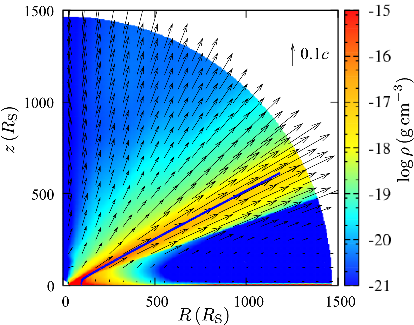
1. UV line-driven winds are more polar than equatorial
(as opposed to other models)
As opposed to Proga 04, Risaliti & Elvis 10, Nomura 16
2. UV line-driven winds get v ~ (0.05 - 0.5) c, with relativistic corrections
As opposed to Luminari 21
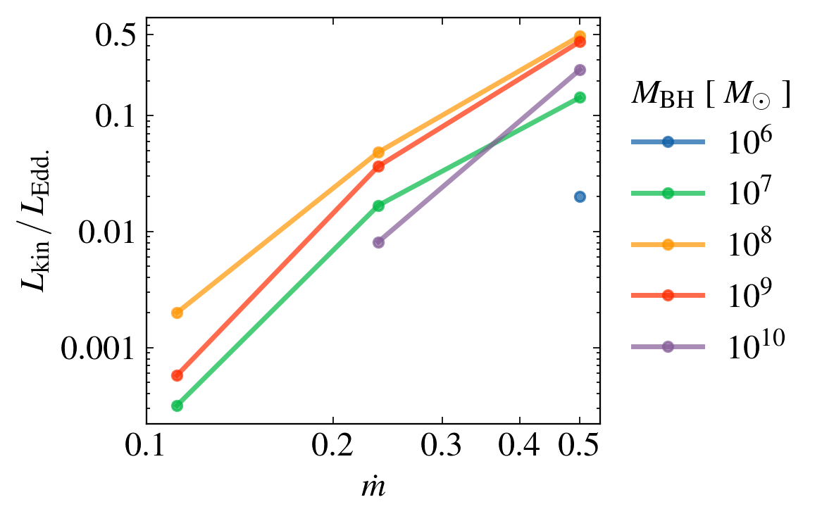
3. UV line-driven winds kinetic luminosity scales as the (3-4)th power of Eddington ratio.
As opposed to cosmological simulations AGN feedback models Schaye 15 (Eagle), Weinberger 18 (IllustrisTNG), Dave 19 (Simba)
*
*Not peer-reviewed, T&C apply.
METHODs
Simulating line-driven winds
Different approaches
Nomura et al (2018)
Hydro
Non-hydro (QWIND)
- Solves hydrodynamics
- Slow
- No gas pressure.
- Very fast
- Steady-state solutions
Risaliti & Elvis 2010, Quera-Bofarull (2020)
The Qwind code
Simulate gas blob trajectories
\vec{a} =
\vec{a}_\mathrm{es} +
\vec{a}_\mathrm{grav}
+
\vec{a}_\mathrm{lines}
UV vs X-rays
Need to shield against X-Rays
\vec{a}_\mathrm{lines}
X-Rays
UV
The Qwind code
Original model limitations include:
- Initial conditions as free parameter
- Simplified radiation transfer (constant density atmosphere, UV optical depth from centre, "colorless" SED...)
- No relativistic corrections to the radiation flux (wind velocity > c in some cases)
The Qwind ROADMAP
Original model
Risaliti & Elvis 2010
Code release
Quera-Bofarull 2020
Qwind3
Quera-Bofarull 2021
- Numerical improvements
- Port to Python
- Self-consistent initial conditions
- Realistic SED and Radiation Transfer
- Relativistic Corrections
- Port to Julia
Improvements to qwind
INITIAL coNDITIONS
Density and velocity at the base of the wind
Model very sensitive to these values:
- How much mass is lifted from the disc
- How much obscuration in the wind
INITIAL coNDITIONS
Idea: Use a 1D solution to approximate them
Close to the disc surface:
a_R \sim 0
R
z
INITIAL coNDITIONS
Think the accretion disc as a collection of O-stars at different temperatures
INITIAL coNDITIONS
1D solution -> O star winds
a_\mathrm{grav}
a_\mathrm{rad}
O stars
Solution is well studied
CAK formalism
Castor, Abbott & Klein (1975)
INITIAL coNDITIONS
We apply the CAK formalism to accretion discs
Pereyra et al. (04, 06)
\rho \frac{dV}{dt} = - \rho \,(a_\mathrm{grav} + a_\mathrm{rad}) - \frac{\partial P}{\partial z}
Compute mass loss at the "critical point"
Get density at the sonic point
INITIAL coNDITIONS
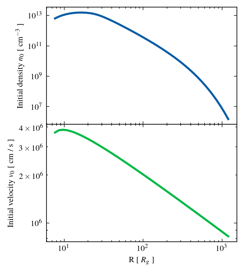
Initial density
Initial velocity
Initial radius
M_\mathrm{BH} = 10^8 M_\odot \\
\dot m = 0.5
INITIAL coNDITIONS
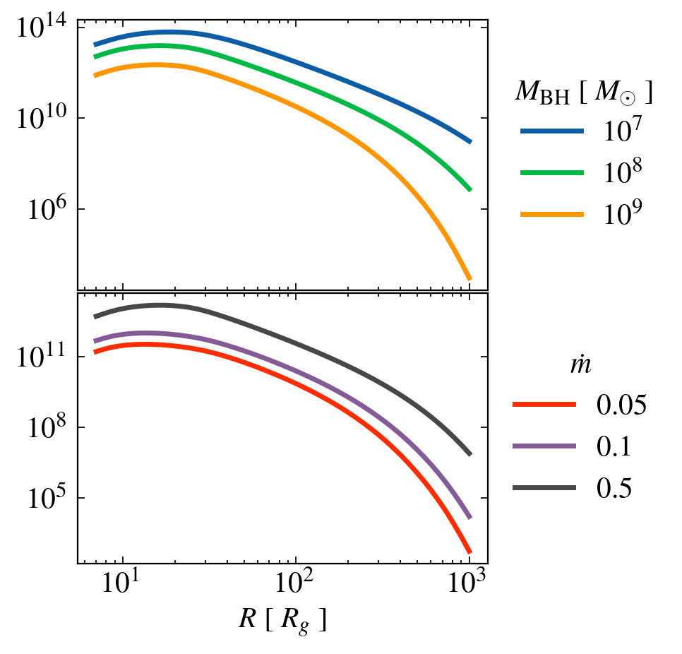
Initial Density [cm^-3]
Radiation Transfer
Two main sources of radiation:
Accretion disc (UV)
Vicinity of the BH (X-ray)
Radiation Transfer
UV source (disc) treatment limitations
- UV power fraction per annulus = const.
UV Fraction with radius
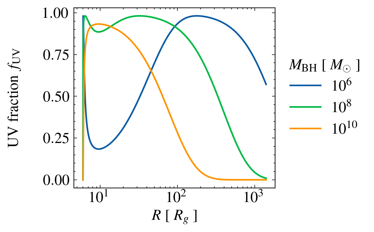
\dot m = 0.5
Interesting physics: this breaks wind properties symmetry on
M_\mathrm{BH}
Radiation Transfer
UV source (disc) treatment limitations
2. Ray tracing through the wind
Original model:
\tau_\mathrm{UV}
\tau_\mathrm{X}
Radiation Transfer
UV source (disc) treatment limitations
2. Ray tracing through the wind
Updated model:
\tau_\mathrm{UV}
\tau_\mathrm{X}
\tau_\mathrm{UV}
\tau_\mathrm{UV}
See Christian Knigge talk for X-ray treatment limitations
Relativistic correction also takes into account the full velocity field
Radiation Transfer
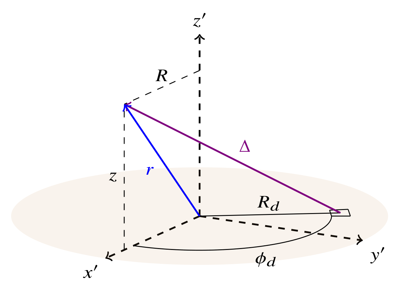
We integrate the disc radiation force mitigating each individual light ray.
Radiation Transfer
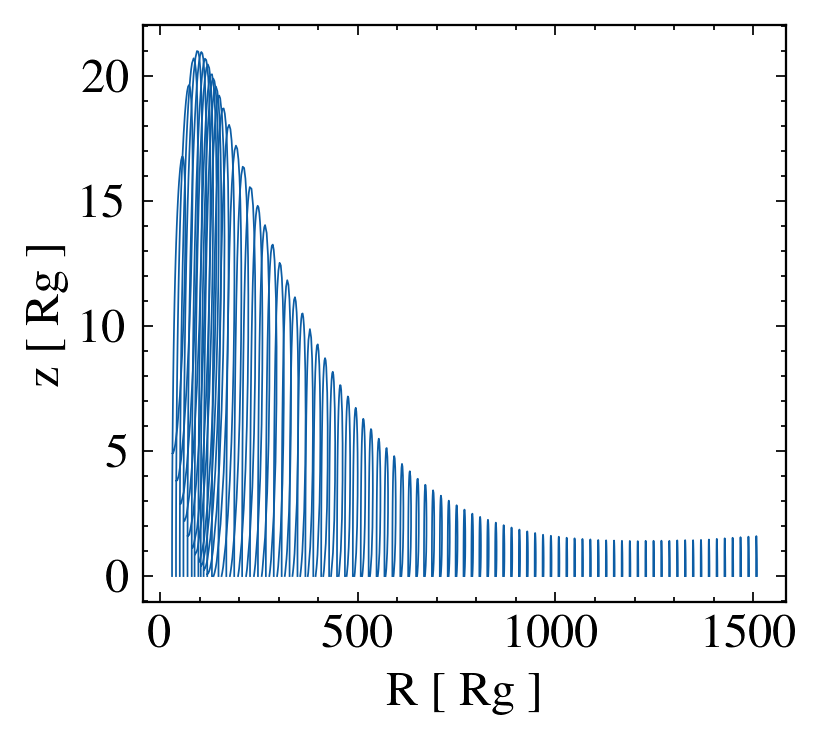
Wind Dynamics
Radiation Transfer
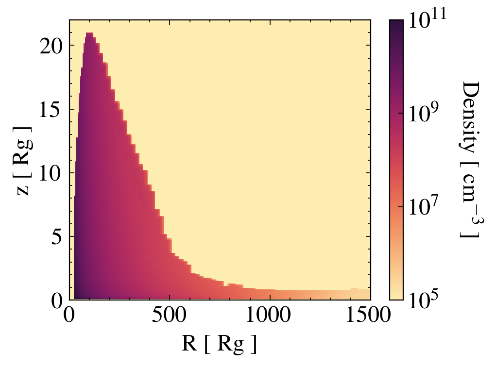
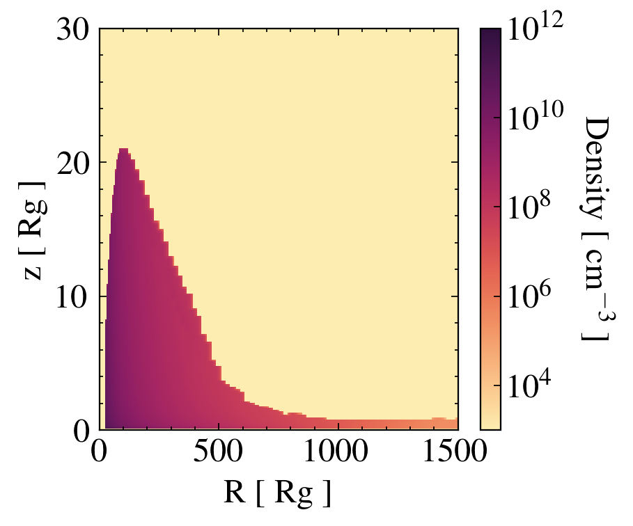
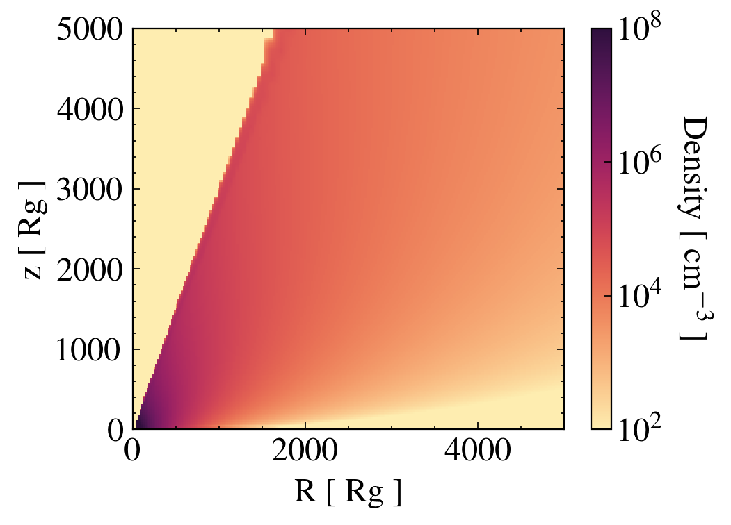
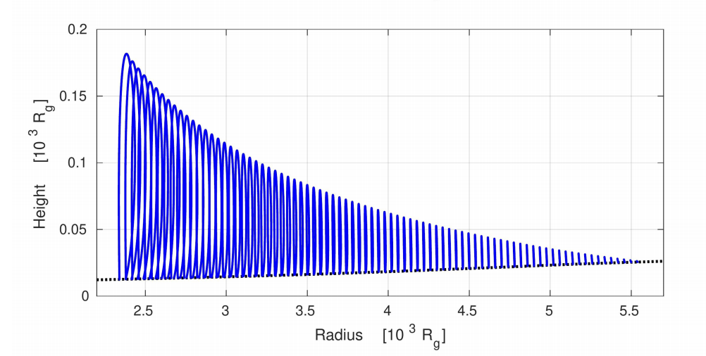
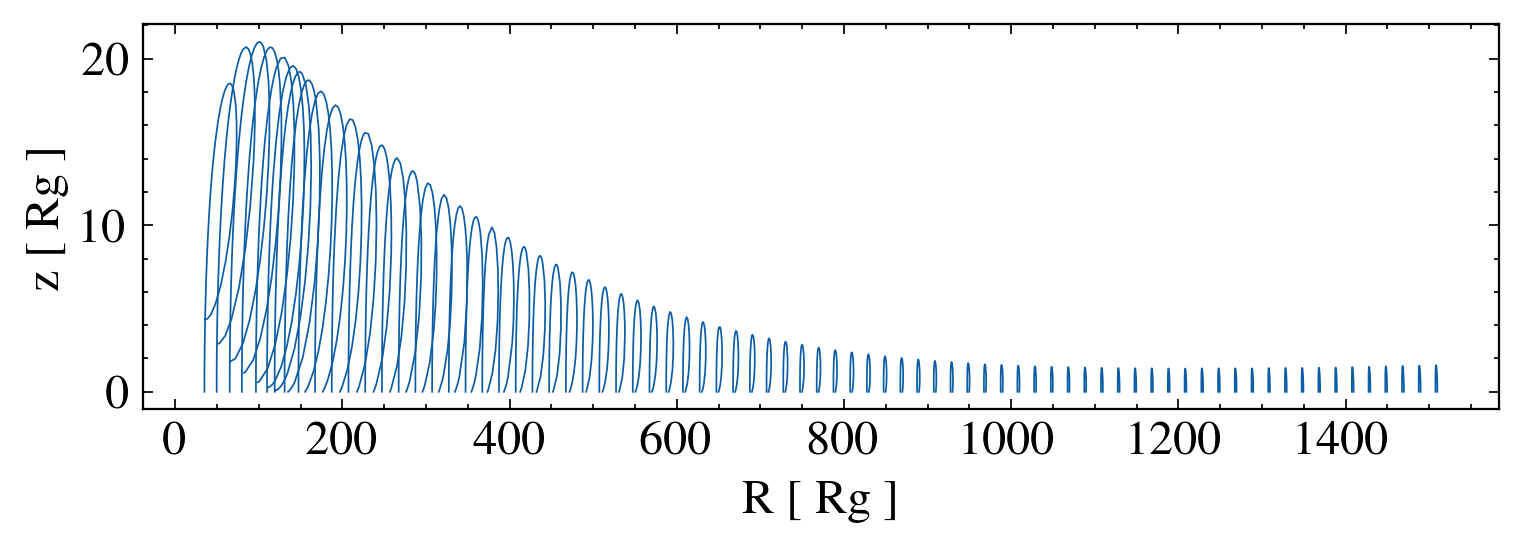
Density field
an iterative approach
1st iteration: Assume vacuum atmosphere.
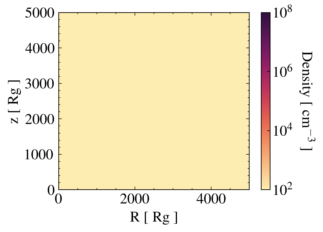
Wind fails because ionisation (no shielding against X-Rays)
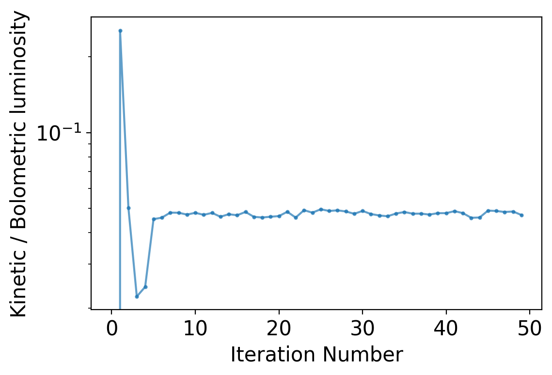
an iterative approach
an iterative approach
an iterative approach
an iterative approach

It converges!
ONE Free parameter left
We know initial density and velocity
At what radius do we start launching the wind?
R_\mathrm{in}
R_\mathrm{in}
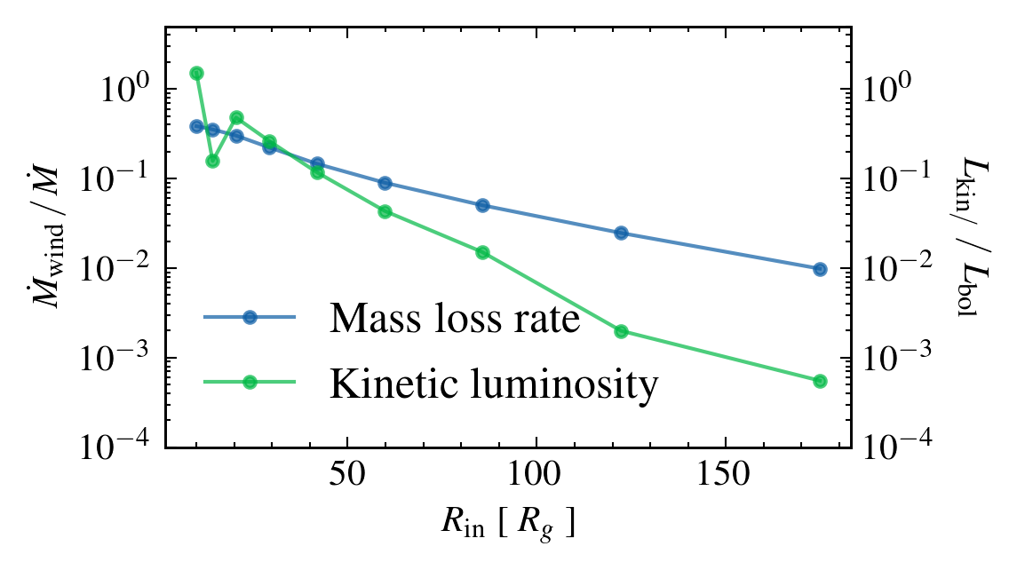
DEPENDENCE ON INITIAL RADIUS
Initial radius (Rg)
Highest UV emission
M_\mathrm{BH} = 10^8 M_\odot \;\; \dot m = 0.5
P04
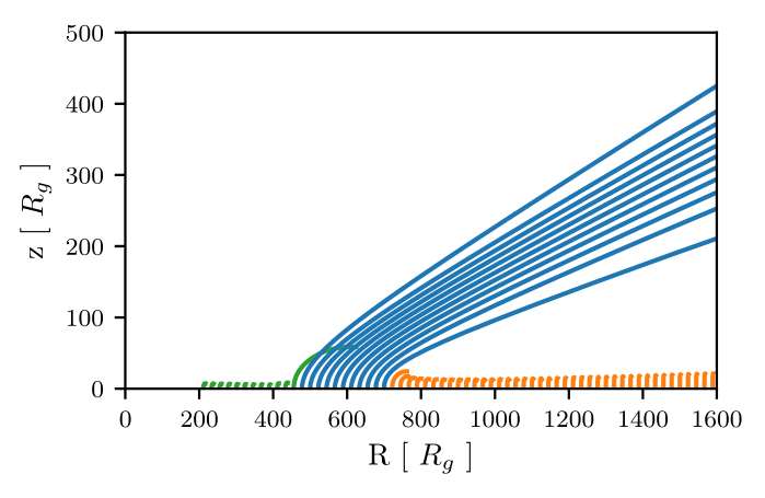
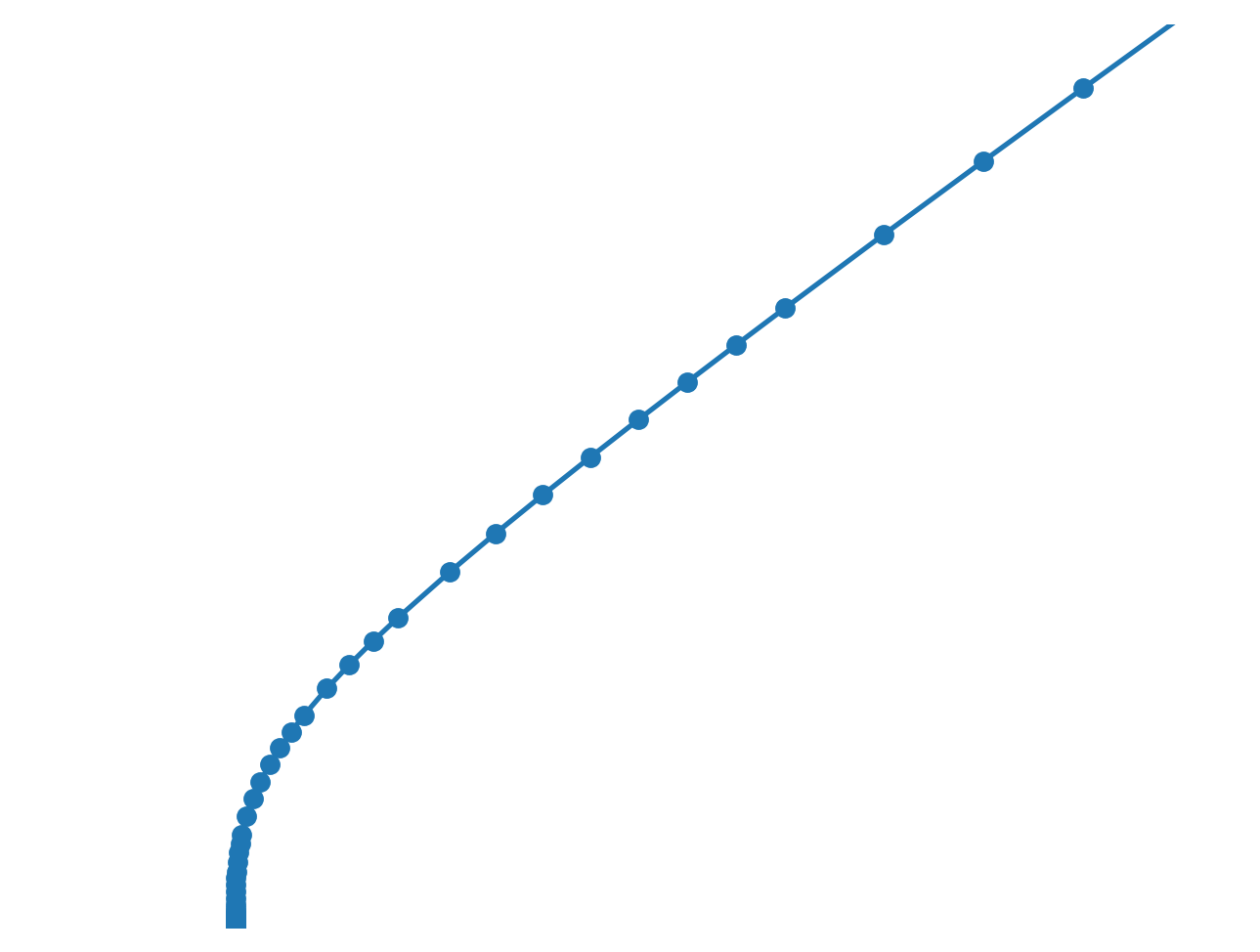
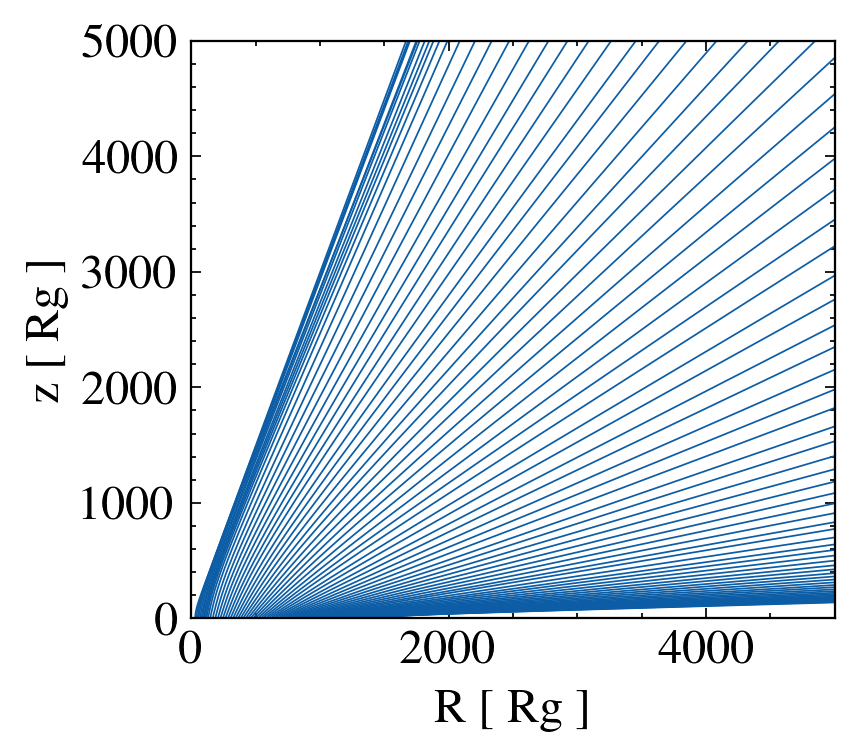
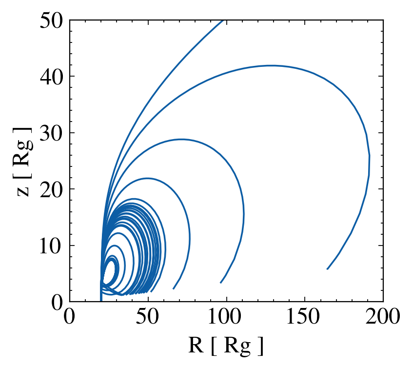
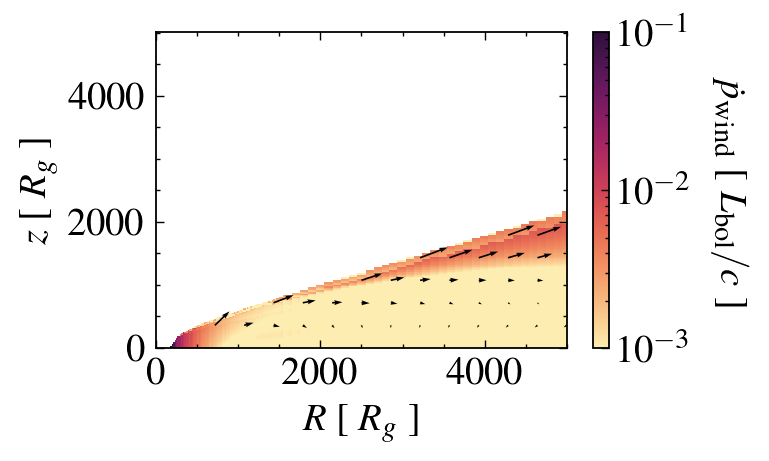
Wind Geometry
Polar or equatorial?
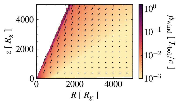
R_\mathrm{in} = 20 \; R_g
R_\mathrm{in} = 100 \; R_g
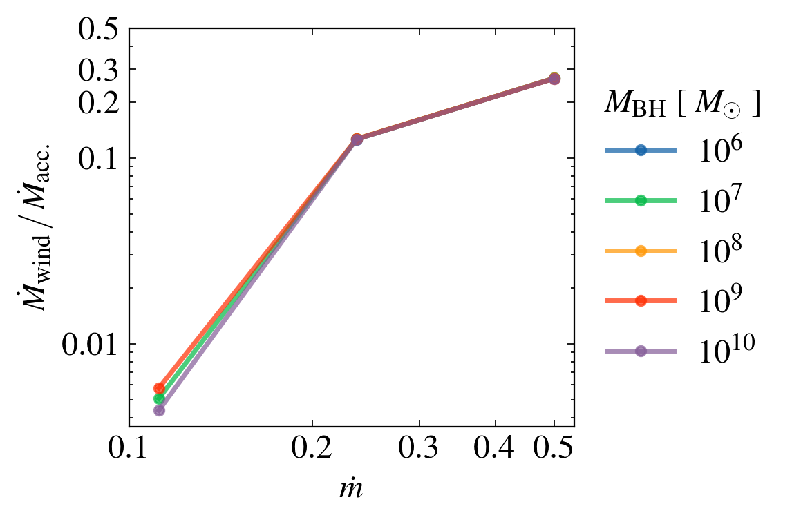
DEPENDENCE on MASS AND MASS ACCRETION RATE
Mass LOss rate
R_\mathrm{in} = 20 R_g
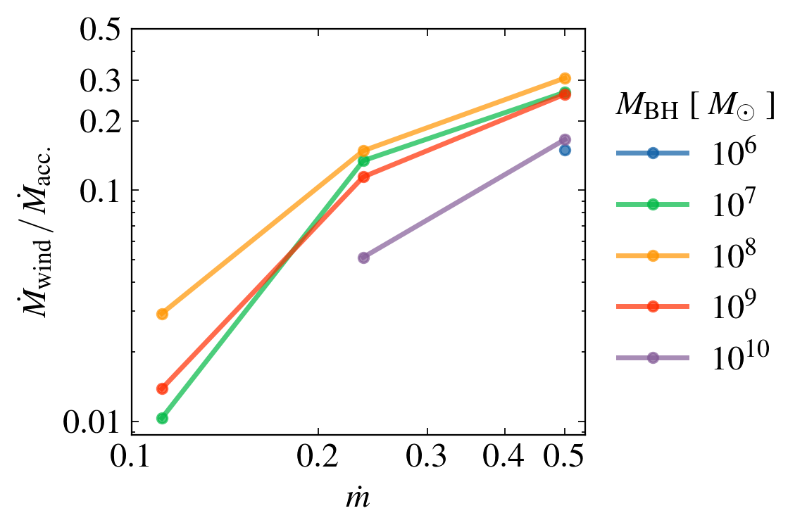
Mass invariant if fuv = constant
R_\mathrm{in} = 20 R_g
DEPENDENCE on MASS AND MASS ACCRETION RATE
KINETIC LUMINOSITY
R_\mathrm{in} = 20 R_g
\frac{L_\mathrm{kin}}{L_\mathrm{Edd}} \sim \dot m^{3-4}
Can uv line-driven winds be ufos?
R_\mathrm{in} = 20 R_g

Can uv line-driven winds be ufos?
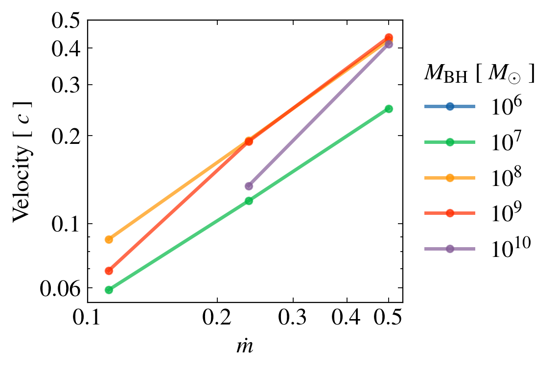
v ~ (0.1 - 0.5) c
even when including relativistic corrections
We do not "need" magnetic winds to generate UFOs.
Different than Luminari 2021
Summary
Slides: www.arnau.space/diskwinds


1. Wind properties heavily dependent on Eddington fraction, weakly dependent on BH mass.
3. Wind can reach up to 0.5c with relativistic corrections
2. Line-driving "natural" range
10^7 - 10^9 M_\odot
BACKUP SLIDES
INITIAL coNDITIONS
Idea: Stable solution passes through the critical point
Critical point defined as the minimum of the nozzle function
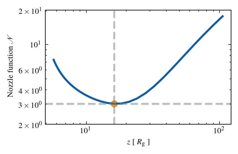
INITIAL coNDITIONS
Critical point
~ Mass loss rate at critical point
INITIAL coNDITIONS
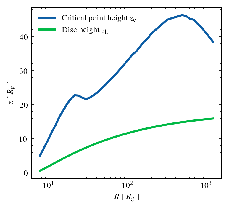
Critical point position
Disc radius
INITIAL coNDITIONS
Critical point position
Mass loss rate (at critical point)
Density and velocity at the sonic point
Use it as our initial state
UV vs X-rays
\vec{a}_\mathrm{lines}
Shielding by failed wind.
Czerny 21
(yesterday's talk)
Qwind
UV line-driven winds:
By arnauqb


