Learning to Deblend Galaxies from Blended Observations with Diffusion Models
Benjamin Remy

at the BDL workshop 3rd edition, Paris, 2025

De-blending galaxies
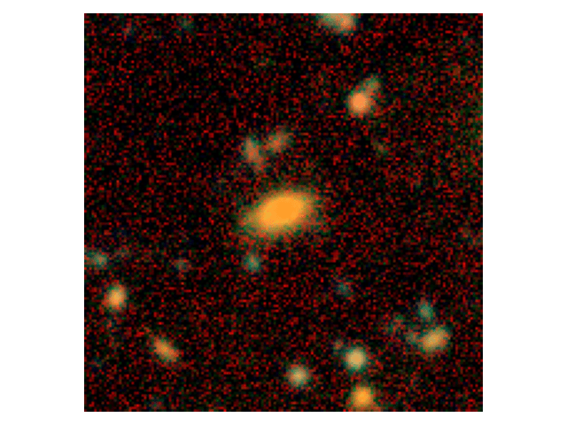
HSC image
Patches contain overlapping sources due to survey depth and large PSF
Need to de-blend galaxies from these images...
PSF convolution, overlapping sources and low SNR makes deblending nontrivial
Blending affects 60% of HSC galaxies (Bosch et al. 2018) and affects their detection and shape measurement

De-blending as an inverse problem
scarlet2
github.com/pmelchior/scarlet2
in JAX, Equinox (differentiable, GPU accetlerated)
- multiband, multi-epochs, multi-resolution
- deep nn prior
- optimization (MAP), sampling (full posterior)


Sampson and Melchior (2024)
Ward et al. (incl. Remy) (2024)
Remy et al. (in prep.)
Siegel and Melchior (2024)
De-blending as an inverse problem
=
+\,\, n
A
\{x_i\}

De-blending as an inverse problem
= \color{white}{A_{\Pi}} \color{white}{\sum_i A_i}
\{x_i\}
Assuming all sources are detected
\color{black}{ =} \color{white}{A_{\Pi}} \color{orange}{\sum_i A_i}
Source mixing

= \color{orange}{A_{\Pi}} \color{black}{\sum_i A_i}
Convolution with the
Point Spread Function

Additive noise
\color{orange}{+ \, \, n}
= \color{black}{A_{\Pi}} \color{black}{\sum_i A_i}
Solving linear inverse problems
y = A_{\Pi} \sum_{i} A_i x_i + n
is ill-posed because
A_{\Pi} \sum_{i} A_i
noise corruption
n
which implies that there are multiple solutions
to the problem
\{x_i\}_N
is not invertible
Solving linear inverse problems
p(\{x_i\}|y) = \dfrac{p(y|\{x_i\})p(\{x_i\})}{p(y)}
Bayes' theorem
Solving linear inverse problems
p(\{x_i\}|y) \propto p(y|\{x_i\})p(\{x_i\})
Bayes' theorem
\propto \color{darkblue}{p(y|\{x_i\})}\color{dark}{\prod_i} \color{darkorange}{p(x_i)}
Likelihood
n \sim \mathcal{N}\left( 0, \Sigma_n\right)
y \sim \mathcal{N}\left( A_{\Pi} \sum_{i} A_i x_i, \Sigma_n\right)
Prior
- Closed form profile
(Expenentional, Sersic, Bulge+disk)
- learned from simulations
x \sim p(x)


Solving linear inverse problems
\underset{x}{\arg \max}\,\,\, p(\{x_i\}|y) = \underset{x}{\arg \max}\,\,\, \color{darkblue}{p(y|\{x_i\})}\color{black}{\prod_i} \color{darkorange}{p(x_i)}
Via optimization with gradient descent
\underset{x}{\arg \min} -\log p(\{x_i\}|y) = \underset{x}{\arg \min} \color{darkblue}{-\log p(y|\{x_i\})} - \color{black}{\sum_i} \color{darkorange}{\log p(x_i)}
This works! But
- targets only the MAP
- requires a good initialization of the sources

Model
Rendered model
Observation
Residuals
Solving linear inverse problems
Via diffusion sampling using the reverse SDE


...
...
...
...
Solving linear inverse problems
Via diffusion sampling using the reverse SDE
dx = \bigl[ f(x, t)-g^2(t)\bigl( \color{darkblue}{\nabla \log p_t(y|\{x_i\})} + \color{black}{\sum_i} \color{darkorange}{\nabla\log p_t(x_i)} \color{black}{ \bigr) \bigr]dt + g(t) dw}

Model
Rendered model
Observation
Residuals
\{x_i\}_t
A \{x_i\}_t
y
y - A \{x_i\}_t
Improving the prior via
Expectation-Maximization
Rozet et al. (2024)
Barco et al. (2024)
\theta_{k+1} = \underset{\theta}{\arg\max}\,\,\, \mathbb{E}_{p(y)} \mathbb{E}_{\color{darkgreen}{p_{\theta_k}(x|y)}} \bigl[ \color{orange}{\log p_\theta(x)} \color{black}{\bigr]},
If the parameters of the prior are updated such as
then converges to a local maximum, and the evidence
is maximized under this model.
p_\theta(x)
p_\theta(y)
1. Sample from the posterior (via diffusion)
\theta
2. Maximize the log prob of the model (via score-matching)
\color{darkgreen}{x \sim p_{\theta_k}(x|y)}
Improving the prior via
Expectation-Maximization
Rozet et al. (2024)
Barco et al. (2024)
On HST images

A \{x_i\}_t
y
y - A \{x_i\}_t
k=0

k=1

k=2

k=3

k=4

k=5

k=6

k=7

k=8

k=9

k=10
Prior initially learned from
scarlet1 fits
Takeways
Upcomming surveys such as LSST will require robust deblending methods to separate overlapping sources in crowded fields
Deblending is a challenging inverse problem due to PSF convolution, noise, and source mixing
Can be addressed with diffusion sampling and optimization with a deep neural network prior, which can be trained directly from the observations
This requires a differentiable foward model of astronomical sources , which is the purpose of scarlet2
Working for multi-bands, multi-epochs, and muti-resolutions (surveys) settings!

Sampson and Melchior (2024)
Ward et al. (incl. Remy) (2024)
Remy et al. (in prep.)
Siegel and Melchior (2024)
github.pmelchior/scarlet2
BDL2025
By Benjamin REMY


