Diffusion model for full field inference: application to weak lensing
Benjamin Remy
Survey Science Group, KICP


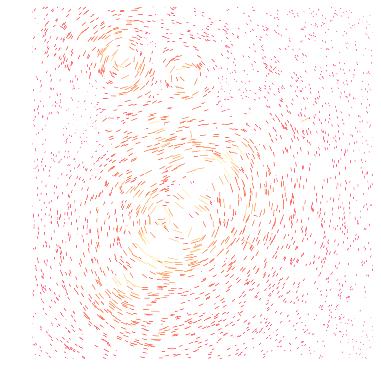
Shear
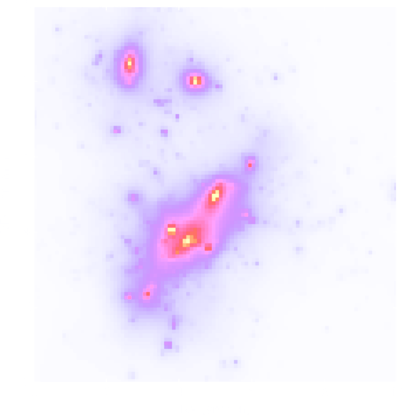
Convergence
\gamma
\kappa
Weak lensing mass-mapping as an inverse problem
\gamma_1 = \frac{1}{2}(\partial_1^2 -\partial_2^2)\Psi
\gamma_2 = \partial_1^2\partial_2^2\Psi
\kappa = \frac{1}{2}(\partial_1^2 + \partial_2^2)\Psi
Shear
Convergence
\gamma
\kappa
Weak lensing mass-mapping as an inverse problem
\gamma = \mathbf{P}\kappa
Mass-mapping with the Dark Energy Survey (DES) Y3
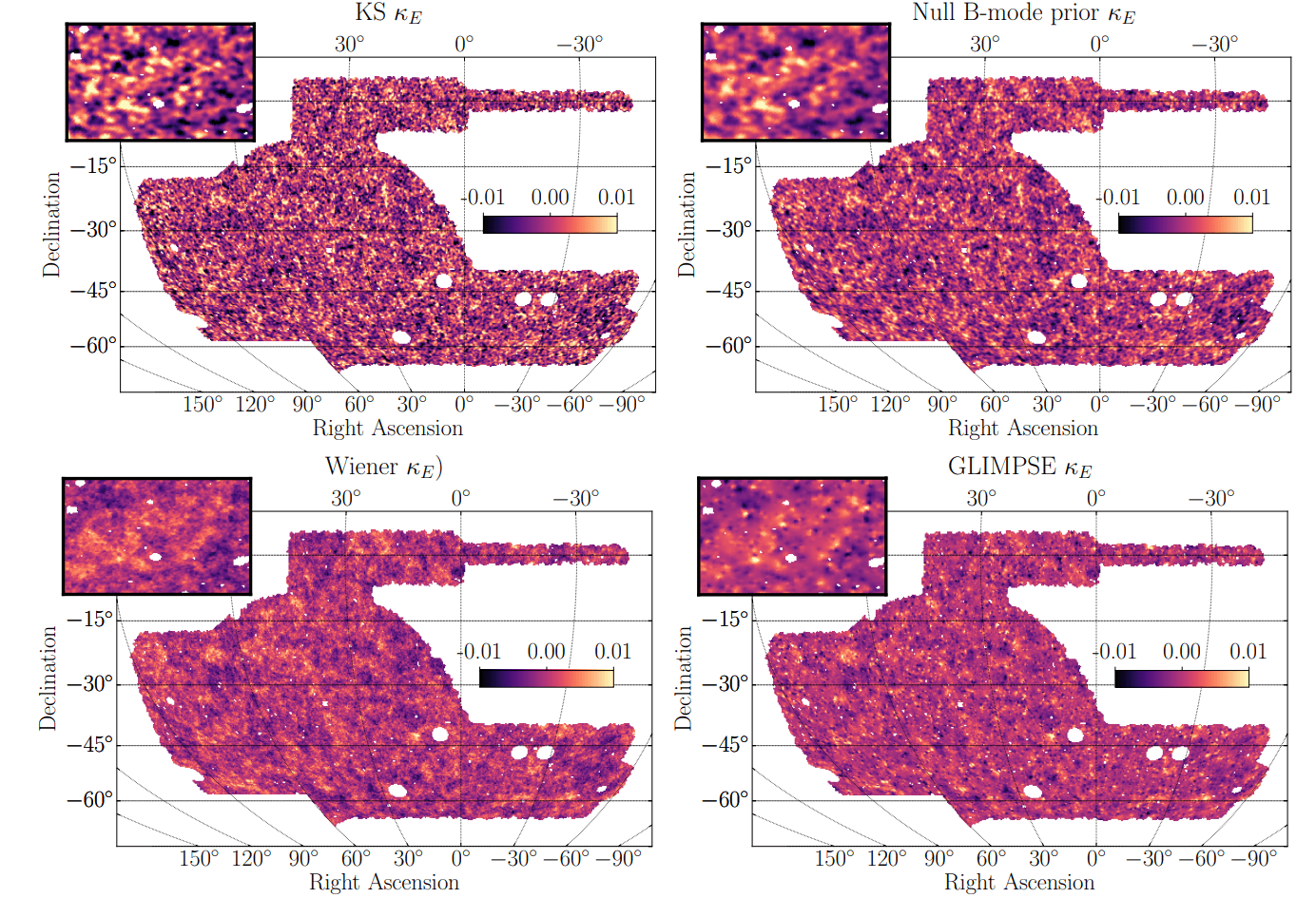
Jeffrey, Gatti, et al. 2021
What about using the prior from cosmological simulations?
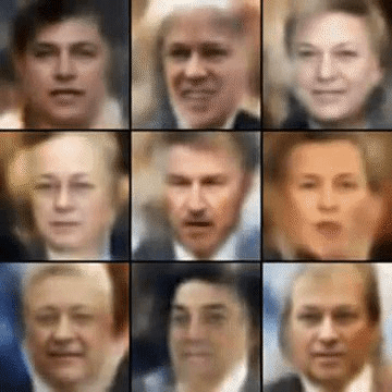
The evolution of generative models
- Deep Belief Network
(Hinton et al. 2006)
The evolution of generative models
- Deep Belief Network
(Hinton et al. 2006)
- Variational AutoEncoder
(Kingma & Welling 2014)
The evolution of generative models
- Deep Belief Network
(Hinton et al. 2006)
- Variational AutoEncoder
(Kingma & Welling 2014)
- Generative Adversarial Network
(Goodfellow et al. 2014), WGAN (2017)
The evolution of generative models
- Deep Belief Network
(Hinton et al. 2006)
- Variational AutoEncoder
(Kingma & Welling 2014)
- Generative Adversarial Network
(Goodfellow et al. 2014), WGAN (2017)
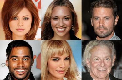
- Diffusion models (Ho et al. 2020, Song et al. 2020)

Midjourney v3
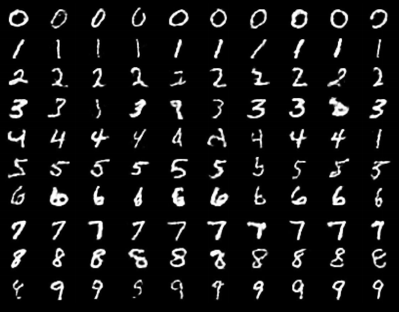
Generative modeling
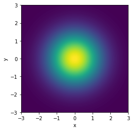
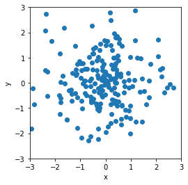
Generative modeling aims to learn an implicit distribution
from which the training set
\mathbb{P}
X = \left\{ x_0, x_1, \dots , x_n \right\}
This usually means building a parametric model that tries to be close to
\mathbb{P}_\theta
\mathbb{P}
\mathbb{P}
x \sim \mathbb{P}
\mathbb{P}_\theta
Model
Samples
True
Once trained, we can typically samples from and evaluate the density
\mathbb{P}_\theta
p_\theta(x)
is drawn.
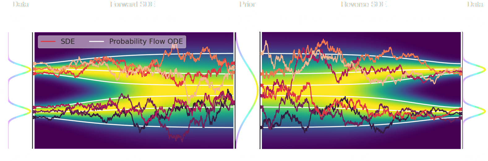
Diffusion models
Once is learned, draw and solve the reverse SDE to get target distribution samples
\nabla \log p(x)
x_T \sim \mathcal{N}(0, \sigma_T)
x_0
The score is all you need
\nabla \log p_t(x)
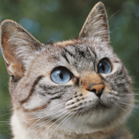
We learn is by denoising our data
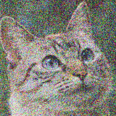
If is corrupted by additional Gaussian noise
x \sim \mathbb{P}
x^\prime = x + n
Then a denoiser trained under an loss
d_\theta(x^\prime, \sigma_t)
\ell_2
\ell_2 = \| x - d_\theta(x^\prime, \sigma_t) \|^2_2
Verifies the Tweedie's formula
\nabla \log p_t(x^\prime) = \frac{d_\theta(x^\prime, \sigma_t) - x^\prime}{\sigma_t^2}

\nabla \log p_t(x^\prime)
x
x + n
n \sim \mathcal{N}(0, \sigma_t)
d_\theta(x^\prime, \sigma_t)
Diffusion models for inverse problems
y = \mathbf{A}x + n
is known and encodes our physical understanding of the problem.
⟹ When non-invertible or ill-conditioned, the inverse problem is ill-posed with no unique solution x
\mathbf{A}
Deconvolution
Inpainting
Denoising
Diffusion models for inverse problems
y = \mathbf{A}x + n
p(x\mid y) \propto p(y\mid x)p(x)
p(y\mid x)
p(x)
\hat x = \arg \underset{x}{\max}\,\, \log p(y\mid x) + \log p(x)
\hat x = \arg \underset{x}{\max}\,\, -\frac{1}{2}\| y - \mathbf{A} \|^2 + \log p(x)
Or, we can aim to sample from the full posterior distribution by MCMC techniques
For instance, if is Gaussian
n
is the data likelihood, which constains the physics
is our prior knowledge on the solution
We can target the Maximum A Posteriori (MAP)
Bayesian view of the problem:
Posterior sampling with diffusion models
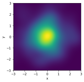
Sampling from the prior
dx = \left[ f(x, t) - g^2(t) \color{yellow}{\nabla_x \log p(x_t)} \right]dt + g(t)dw
p(x)
\kappa\sim p(\kappa)
Posterior sampling with diffusion models
Sampling from the posterior
dx = \left[ f(x, t) - g^2(t) \color{yellow}{\nabla_x \log p(x_t\mid y)} \right]dt + g(t)dw
p(x\mid y)
\color{yellow}{\nabla_x \log p(x_t\mid y)}\, \color{white}{= \nabla_x \log p(y\mid x_t) + \nabla_x \log p(x_t)}
\color{yellow}{\nabla_x \log p(x_t\mid y)}\, \color{white}{= \nabla_x\, \underset{-\frac{1}{2\sigma^2} \| y-\mathbf{A}x \|^2}{\underbrace{\log p(y\mid x_t)}} \,+}\, \color{orange}{\underset{\text{learned}}{\underbrace{\nabla_x \log p(x_t)}}}
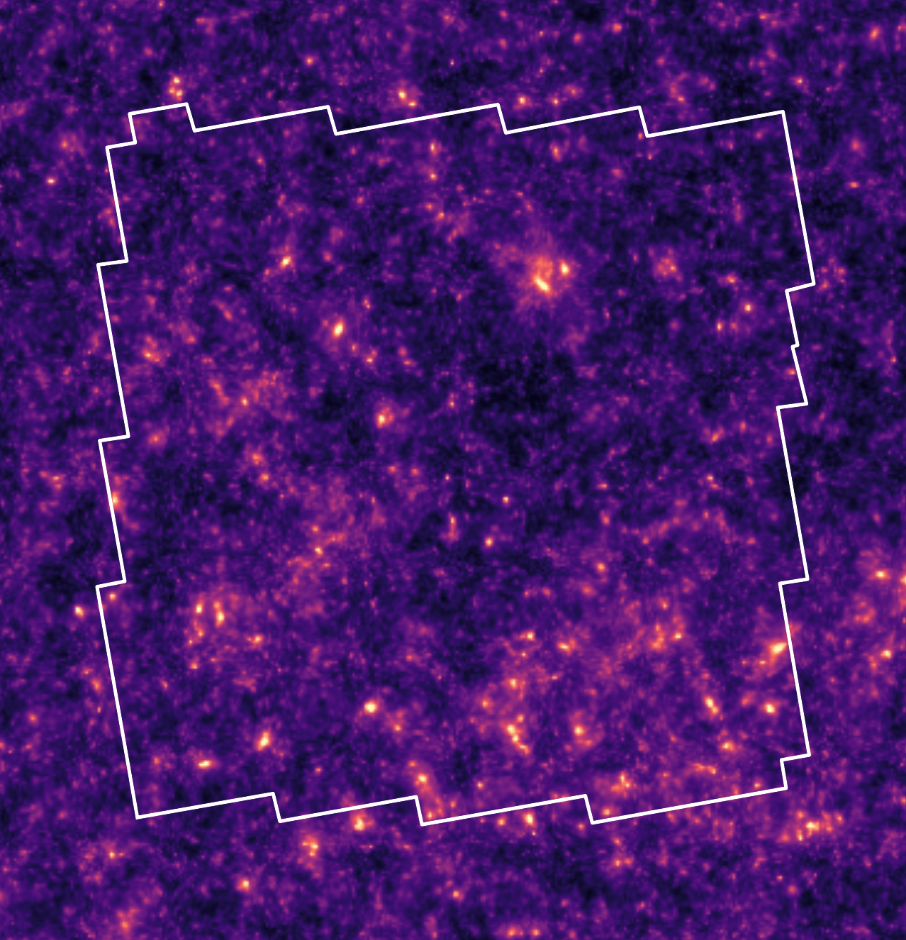
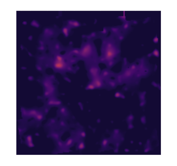
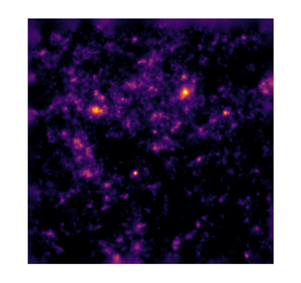
Ground truth simulation
Posterior samples
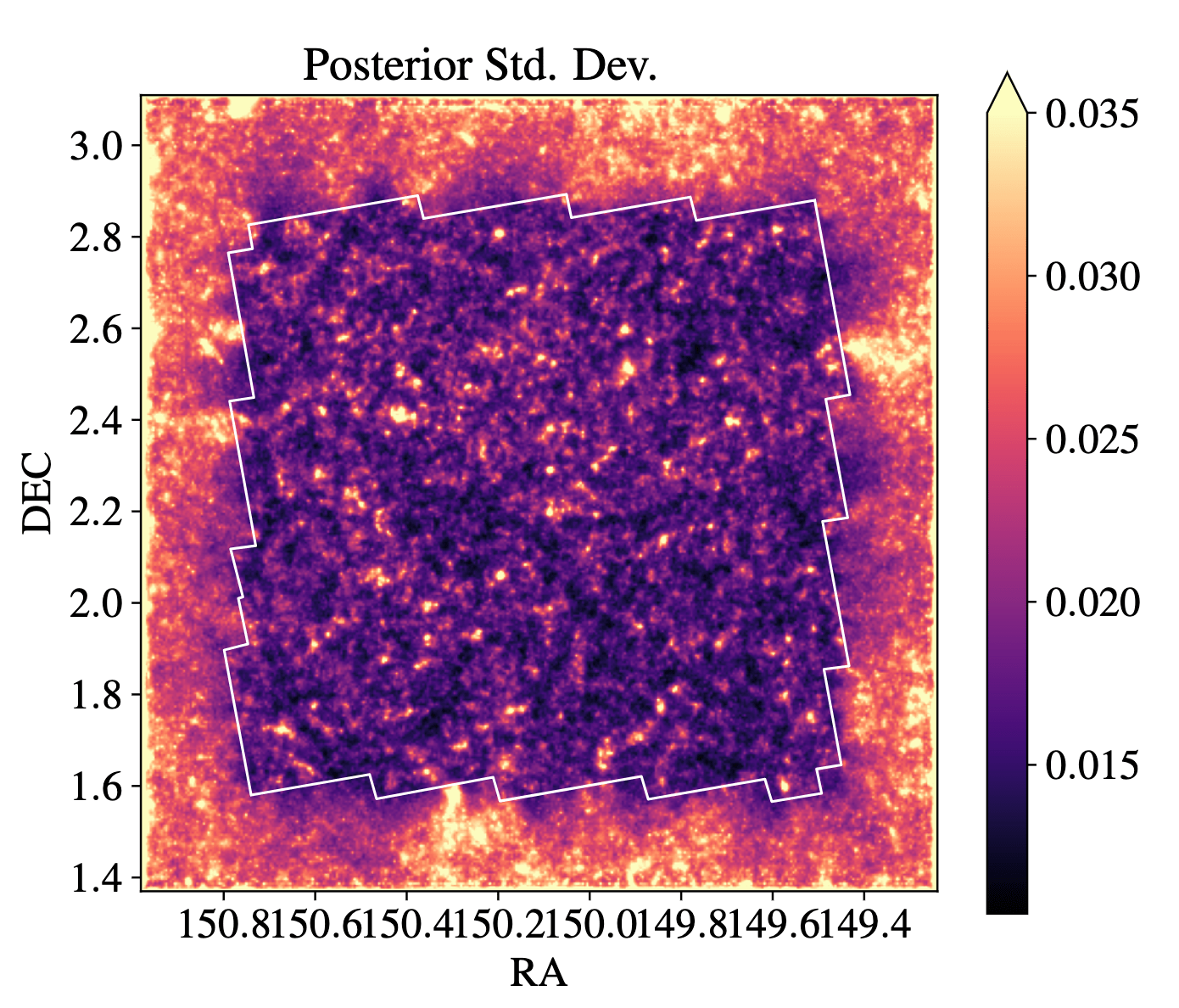
Posterior sampling with diffusion models
Application to HST/ACS COSMOS field
Massey et al. 2007
Remy et al. 2022 (Posterior mean)
Remy et al. 2022 (Posterior samples)
Posterior sampling with diffusion models
Remy et al. 2022 (Posterior mean)
We built a generative model of mass-maps, that we can condition on observation to get the full posterior distribution
p(\kappa\mid \gamma)
But we implicitly assumed a cosmological model when training our prior , i.e.
p(\kappa)
p(\kappa\mid \mathcal{M})
How to infer jointly the cosmology and the mass map?
But we implicitly assumed a cosmological model when training our prior , i.e.
Benjamin Remy, Francois Lanusse, Niall Jeffrey, Jia Liu, Jean-Luc Starck,
Ken Osato, Tim Schrabback, Probabilistic mass-mapping with neural score estimation, A&A 2022
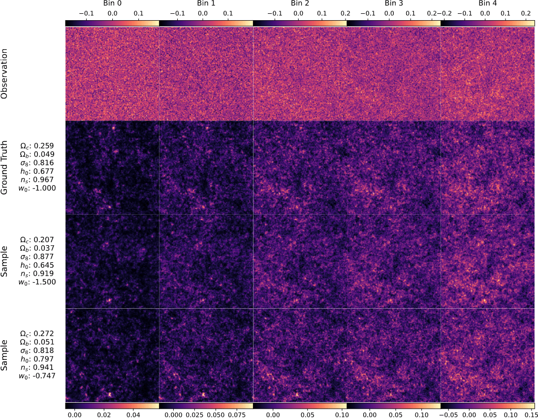
Joint inference of mass-maps and cosmological parameters
with Chihway Chang and Rebecca Willet
Learning the joint distribution
p(\theta, \kappa)

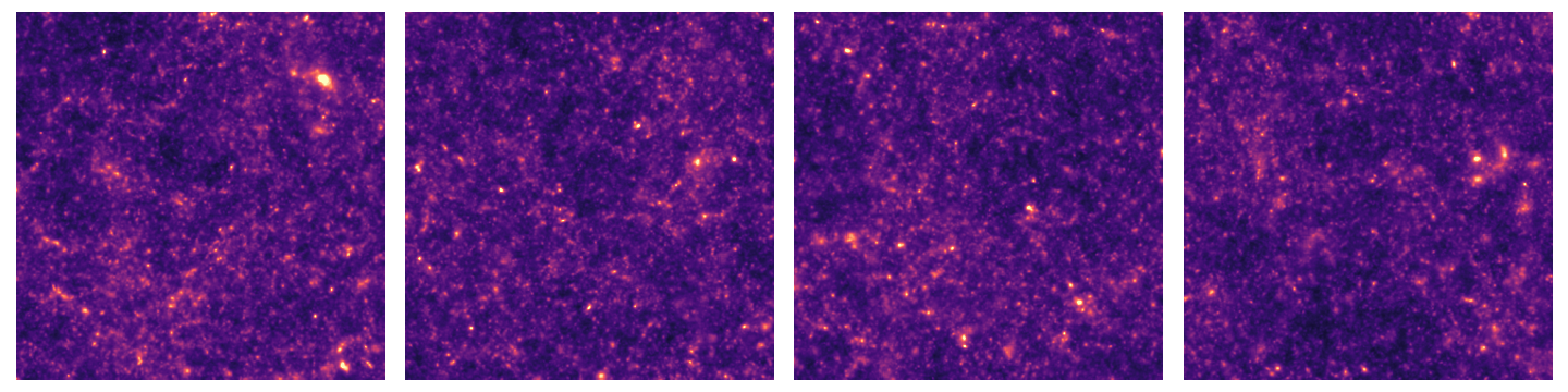
We now have a dataset of pairs
\theta, \kappa \sim p(\theta)p(\kappa\mid \theta)
\theta_0, \kappa_0
\theta_1, \kappa_1
\theta_2, \kappa_2
\theta_3, \kappa_3
How can we build a diffusion model to learn the joint distribution?
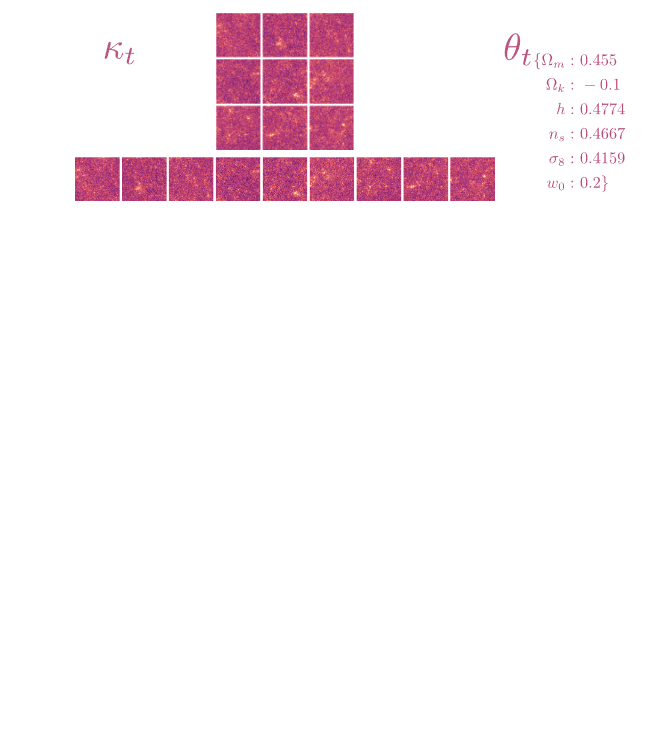
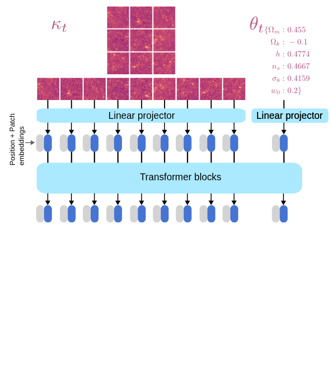
Learning the joint distribution
p(\theta, \kappa)
We need to model to design a denoiser architecture
to learn the score function
\nabla \log p(\theta, \kappa)
\left[\theta^\prime, \kappa^\prime\right] = \left[\theta, \kappa\right] + \sigma_tn
d^\star(\theta^\prime, \kappa^\prime, \sigma_t) = \left[\theta^\star, \kappa^\star\right]
We want to learn the denoiser
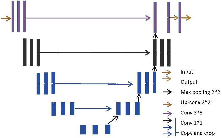
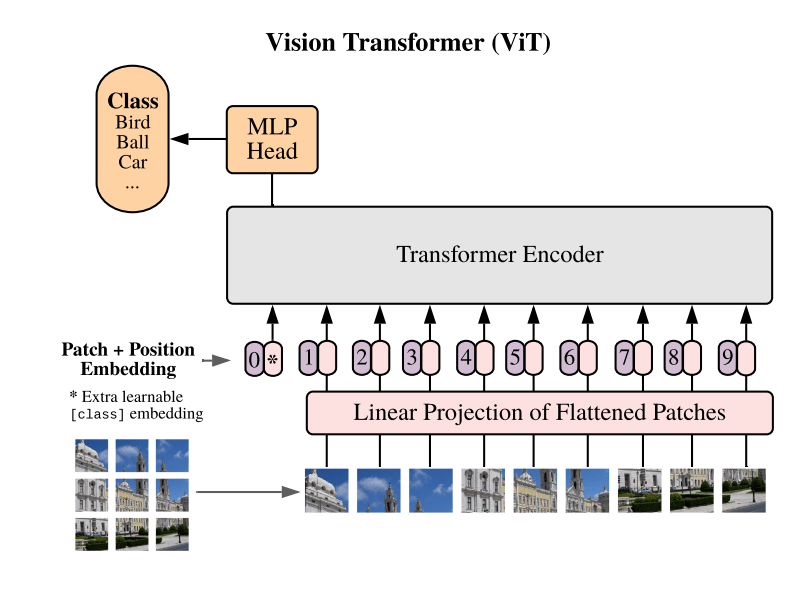
U-net architecture based on convolutional layers
Only inputs and ouputs images (or volumes)....
How do we add the cosmology?
\nabla \log p(\theta, \kappa)
Use Tweedie's formula to get
p(\theta, \kappa)
Learning the joint distribution
p(\theta, \kappa)
We need to model to design a denoiser architecture
to learn the score function.
\left[\theta_t, \kappa_t\right] = \left[\theta, \kappa\right] + \sigma_tn
d^\star(\theta_t, \kappa_t, \sigma_t) = \left[\theta^\star, \kappa^\star\right]
We want to learn the denoiser
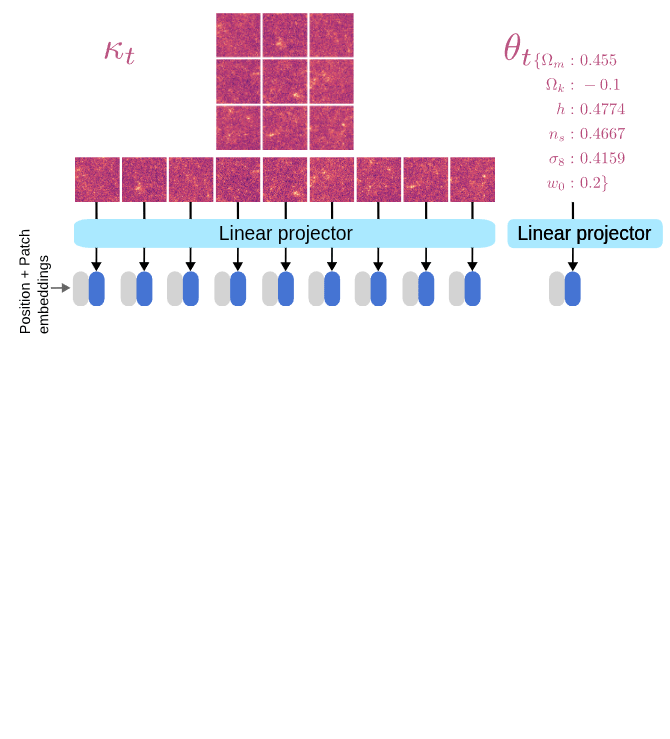
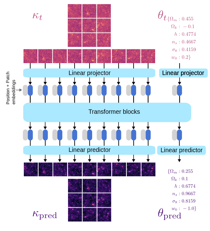
We now have a joint score function!
\nabla_{\kappa, \theta} \log p(\kappa, \theta)
Learning the joint distribution
p(\theta, \kappa)

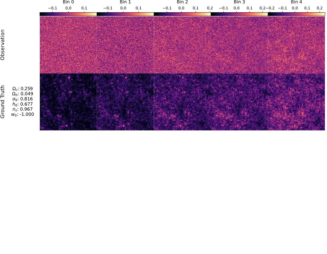
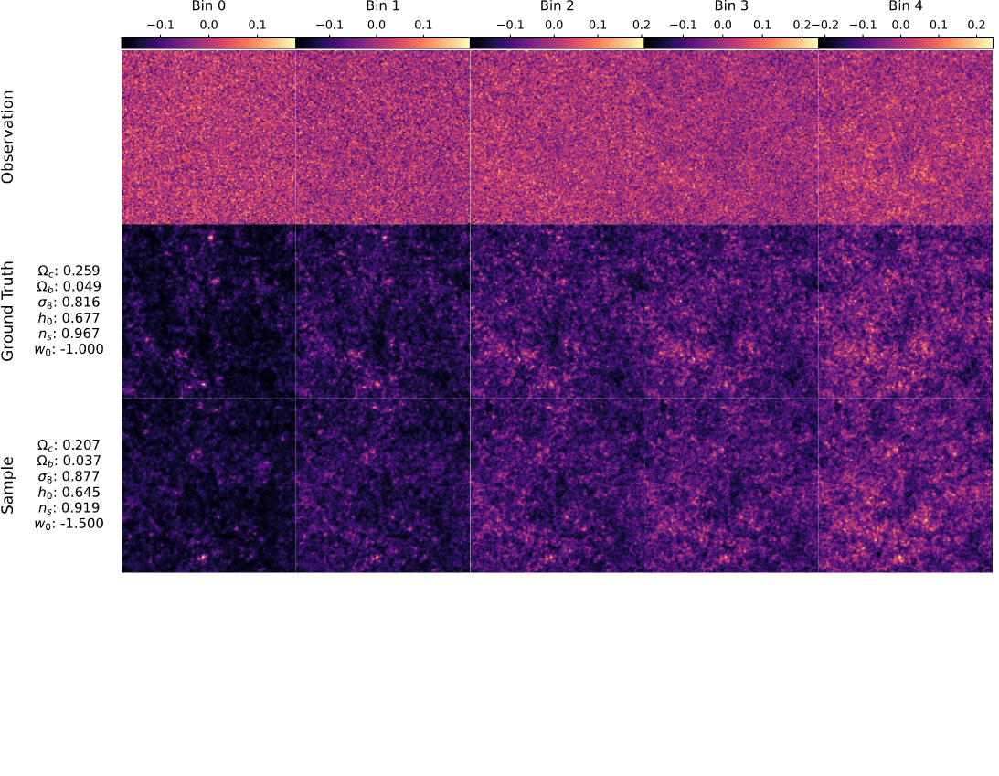
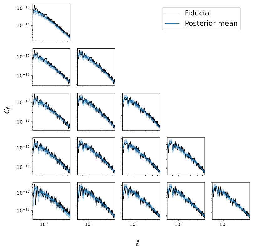
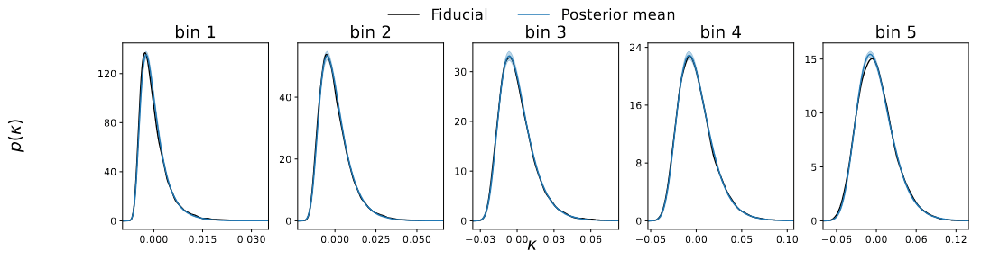
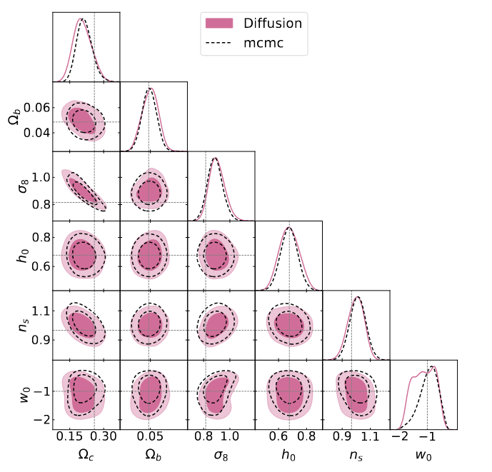
Marginal
p(\theta\mid \gamma)
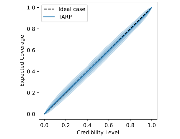
Coverage test
We built a generative model of mass-maps and cosmology, that we can condition on observation to get the joint posterior distribution
p(\theta, \kappa\mid \gamma)
Paper out soon...
Thank you!
Generative models for full field inference
By Benjamin REMY


