Bridging Simulators with Conditional Optimal Transport
Justine Zeghal, Benjamin Remy,
Yashar Hezaveh, François Lanusse, Laurence Perreault-Levasseur


Fast simulations
Full N-body
O(ms) runtime
differentiable
O(ms) runtime -> O(days)
differentiable
✅
✅
✅
❌
❌
❌
realistic
❌
realistic
✅
\log p(x)
\log p(x)
Cosmological simulations
e.g. log-normal, LPT, PM
e.g. full nbody, hydro, etc.
Wrong models generate biases
Full field inference from WL convergence maps
Wrong models generate biases
Full field inference from WL convergence maps
How to learn
the correction ?
x_0
x_1 = \phi(x_0)
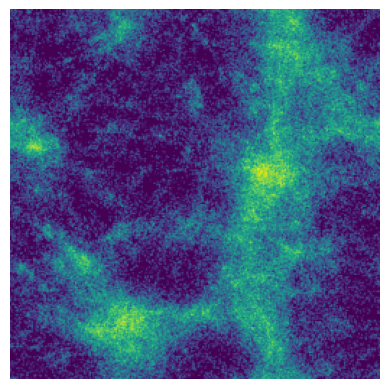
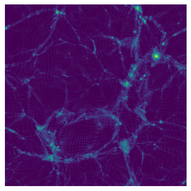
Learning a mapping between simulations
log-normal
from N-body
we seek a minimal transformation so that
the initial conditions and the cosmology are conserved
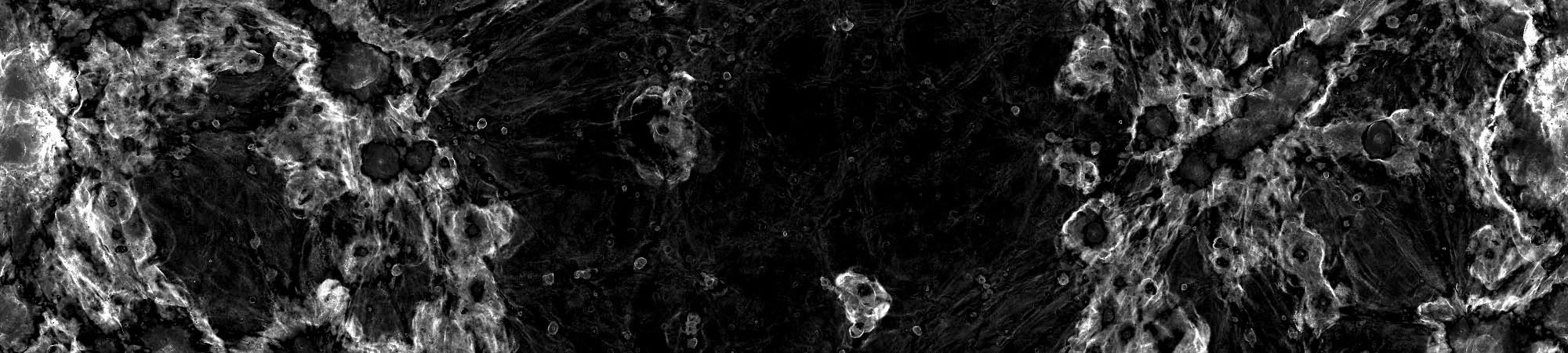
Convergence maps
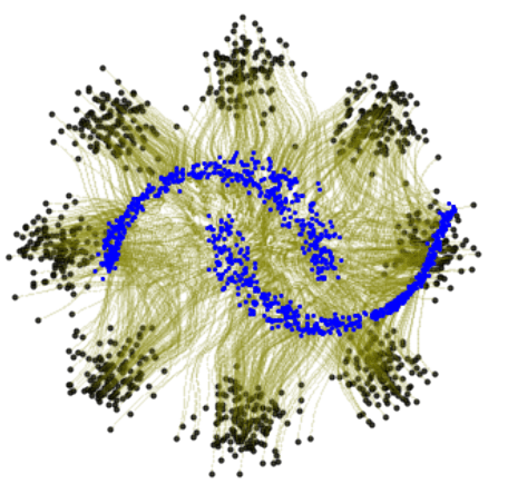
Flow matching for mapping distributions

Flow matching enables us to transport probability distributions in high dimension, using probability flow ODEs
x_0 \sim p_0
x_1 \sim p_1
x_t \sim p_t
\frac{d x_t}{dt} = \color{green}{v_\varphi}\color{black}{(x_t, t)}
Flow matching for mapping distributions
Flow matching enables us to transport probability distributions in high dimension, using probability flow ODEs
x_0 \sim p_0
x_1 \sim p_1
x_t \sim p_t
\frac{d x_t}{dt} = \color{green}{v_\varphi}\color{black}{(x_t, t)}
It can be seen as a continuous normalizing flow but much easier to train:
\mathcal{L}_{FM}(\theta) = \mathbb{E}_{p(t)p(x_0)p(x_1)} \Big[ \| \color{green}{v_\varphi} \color{black}{(x_t, t)- (x_1 - x_0) \|^2 \Big]}
x_t = (1-t)x_1 + t x_0
x_0 \sim p_0, \quad x_t = x_0 + \int_0^t v_\varphi(x, s)ds
\log p_t(x_t) = \log p_0(x_0) - \int_0^t \text{div}\, v_\varphi(x_s) \, ds
x_0 \sim p_0
\color{blue}{x_1 \sim p_1}
Flow matching with optimal transport
p(x_1, x_0) = p(x_1)p(x_0)
\text{mb-OT}(x_1,x_0)
\mathcal{L}_{FM}(\theta) = \mathbb{E}_{p(t)p(x_0, x_1)} \Big[ \| \color{green}{v_\varphi} \color{black}{(x_t, t)- (x_1 - x_0) \|^2 \Big]}
x_t = (1-t)x_1 + t x_0
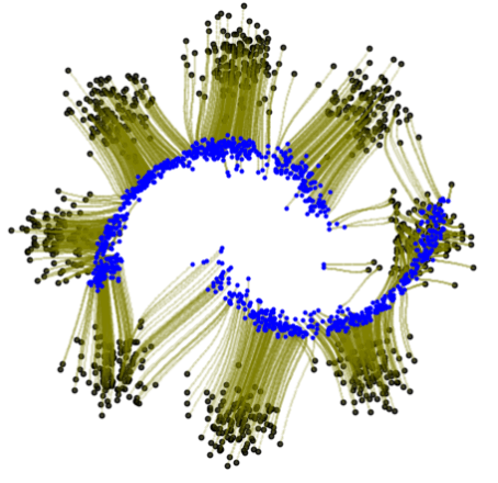
Optimal Transport Flow Maching
Independent coupling
Minibatch OT
OT pairs are found minimizing a quadratic cost
\|x_1 - x_0 \|^2
x_0 \sim p_0
\color{blue}{x_1 \sim p_1}
Flow matching with optimal transport
\text{mb-OT}(x_1,x_0)
\mathcal{L}_{FM}(\theta) = \mathbb{E}_{p(t)p(x_0, x_1)} \Big[ \| \color{green}{v_\varphi} \color{black}{(x_t, t)- (x_1 - x_0) \|^2 \Big]}
x_t = (1-t)x_1 + t x_0
Optimal Transport Flow Maching
Minibatch OT
This coupling solve the problem
W(q_0, q_1)^2_2 = \inf_{p_t, v_t} \int_{\mathbb{R}^d}\int^1_0 p_t(x)\|v_t(x)\|^2 dt dx
i.e. minimizes the path for all trajectories between and
p_0
p_1
Flow matching with optimal transport
OT Flow Matching is helpful because we only care about learning a correction!
\phi
x_0
x_1
Conserving the initial conditions
Flow matching with optimal transport
OT Flow Matching is helpful because we only care about learning a correction!
\phi
x_0
x_1

Dataset 1
Dataset 2
Conserving the initial conditions
Flow matching with optimal transport
Optimal
Transport Plan
\pi(x_0, x_1)
Dataset 1
Dataset 2
OT Flow Matching is helpful because we only care about learning a correction!
\phi
x_0
x_1
Conserving the initial conditions
How to correct while conserving the cosmology?
Flow matching with
conditional optimal transport
(\Omega_{m,0} \; S_{8, 0})
\theta_0
x_0
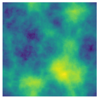
Log-normal
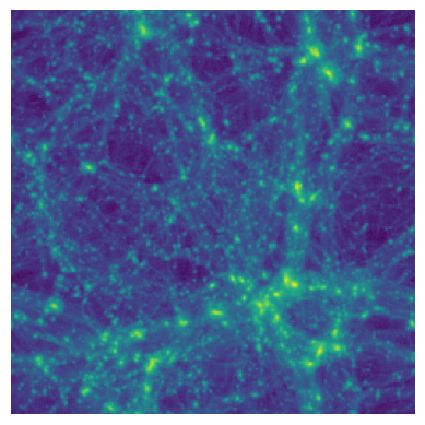
N-body
(\Omega_{m,1} \; S_{8, 1})
\theta_1
x_1
We aim to transport
p(x_1|\theta)
p(x_0|\theta)
to
, i.e. conserving the cosmology
OT FM enables us to transport
p(x_1)
p(x_0)
to
We have two unpaired datasets of
(\theta, x)
We have two unpaired datasets of
(\theta, x)
(\Omega_{m,0} \; S_{8, 0})
\theta_0
x_0
Log-normal
N-body
(\Omega_{m,1} \; S_{8, 1})
\theta_1
x_1
We aim to transport conditionals
p(x_1|\theta)
p(x_0|\theta)
to
, conserving the cosmology
x_t = (1-t)x_1 + t x_0
\mathcal{L}_{FM}(\theta) = \mathbb{E}_{p(t)p(x_0, x_1)} \Big[ \| \color{green}{v_\varphi} \color{black}{(x_t, t)- (x_1 - x_0) \|^2 \Big]}
Flow matching with
conditional optimal transport
(\Omega_{m,0} \; S_{8, 0})
\theta_0
x_0
Log-normal
N-body
(\Omega_{m,1} \; S_{8, 1})
\theta_1
x_1
\mathcal{L}_{FM}(\theta) = \mathbb{E}_{p(t)\color{#3d85c6}{\pi(x_0, x_1)}} \Big[ \| \color{green}{v_\varphi} \color{black}{(x_t, \theta, t)- (x_1 - x_0) \|^2 \Big]}
x_t = (1-t)x_1 + t x_0
Kerrigan et al. 2024: triangular velocity field
\color{green}{v_\varphi\left[\begin{matrix} \theta \\ x \end{matrix}\right] = \left[\begin{matrix} v_\varphi(\theta, t) \\ v_\varphi(\theta, x, t) \end{matrix}\right] = \left[\begin{matrix} 0 \\ v_\varphi(\theta, x, t) \end{matrix}\right]}
finding OT mini-batches by minimizing the joint cost
\color{#3d85c6}{\|\theta_1 - \theta_0 \|^2 + \epsilon \|x_1 - x_0 \|^2}
We have two unpaired datasets of
(\theta, x)
We aim to transport conditionals
p(x_1|\theta)
p(x_0|\theta)
to
, conserving the cosmology
Flow matching with
conditional optimal transport
Fast simulations
Emulated Full N-body
O(ms) runtime
differentiable
O(ms) runtime -> O(days)
differentiable
✅
✅
✅
realistic
❌
realistic
✅
\log p(x)
\log p(x)
Cosmological simulations emulation
e.g. log-normal, LPR, PM
e.g. full nbody, hydro, etc.
\phi
Learned
correction
✅
✅
✅
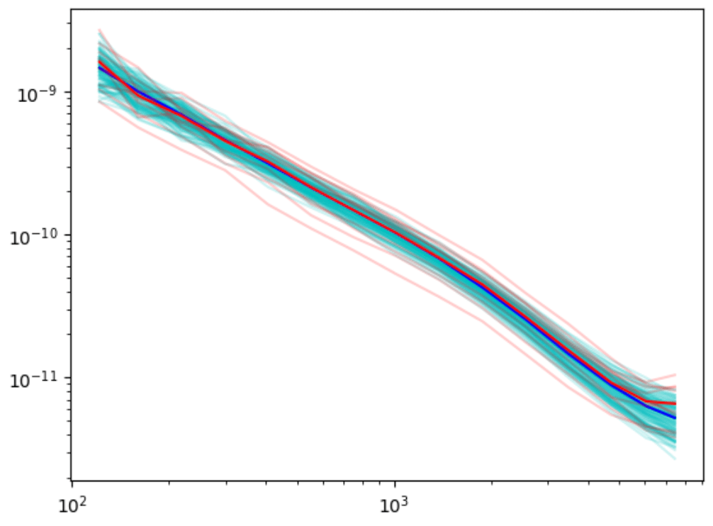
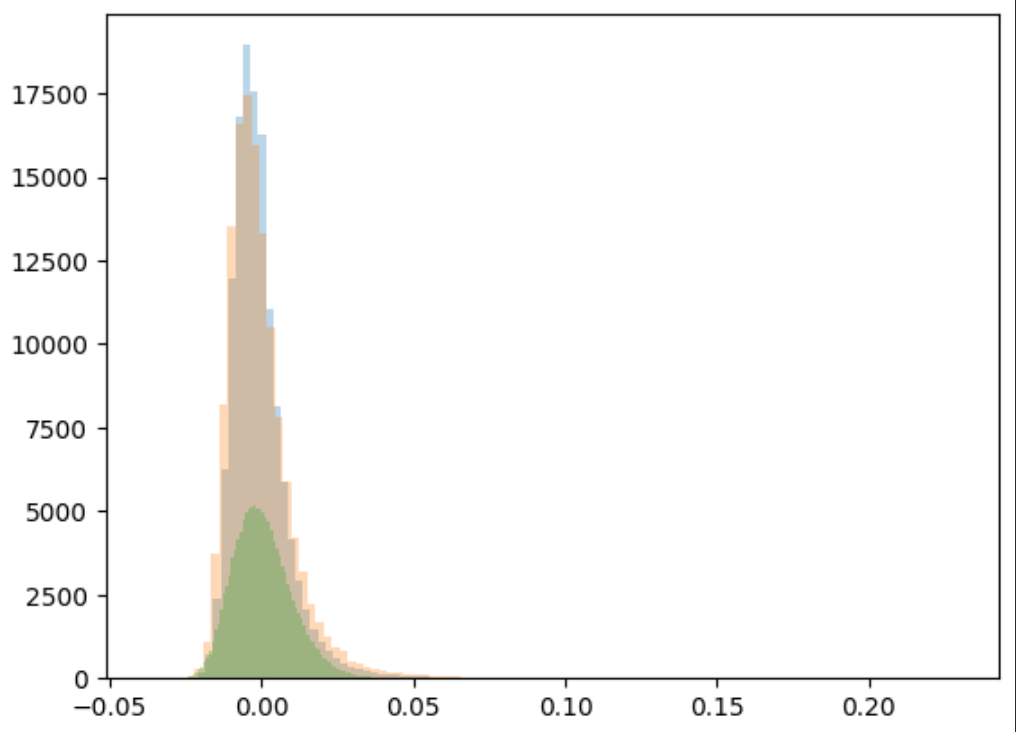
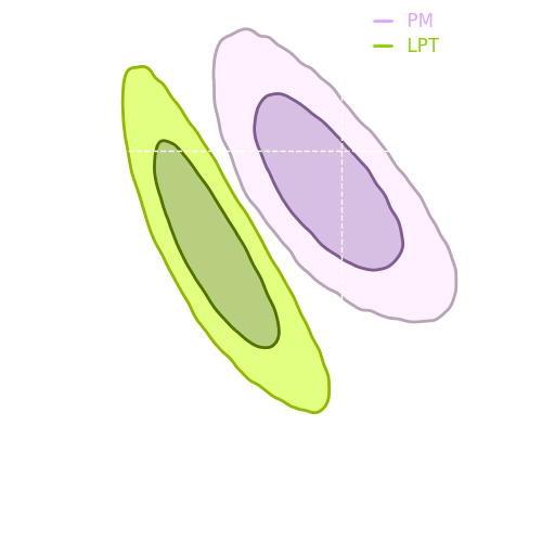
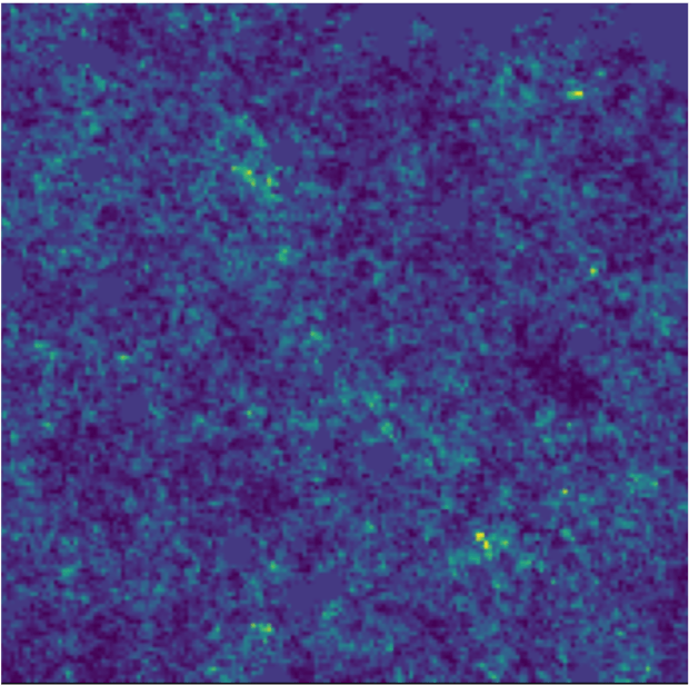
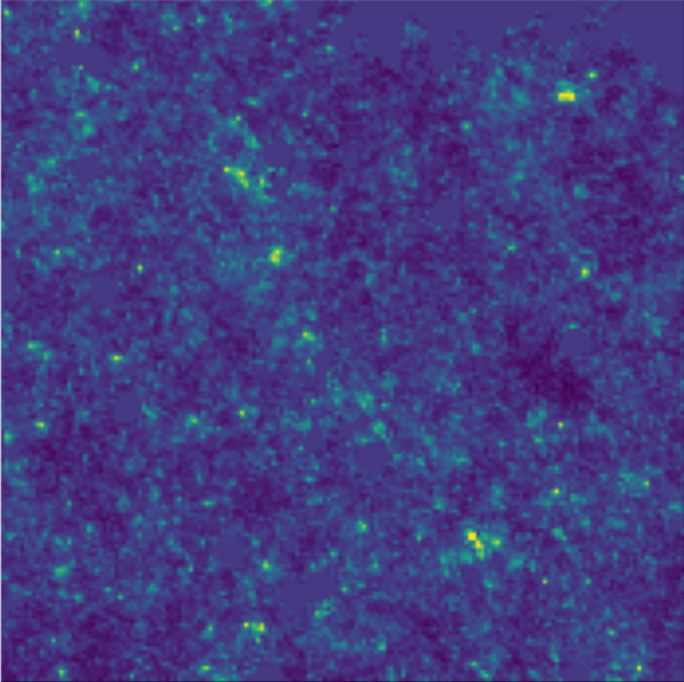
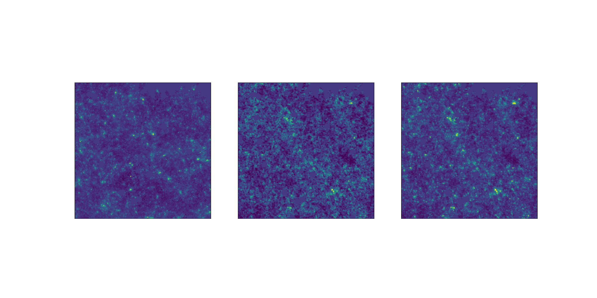
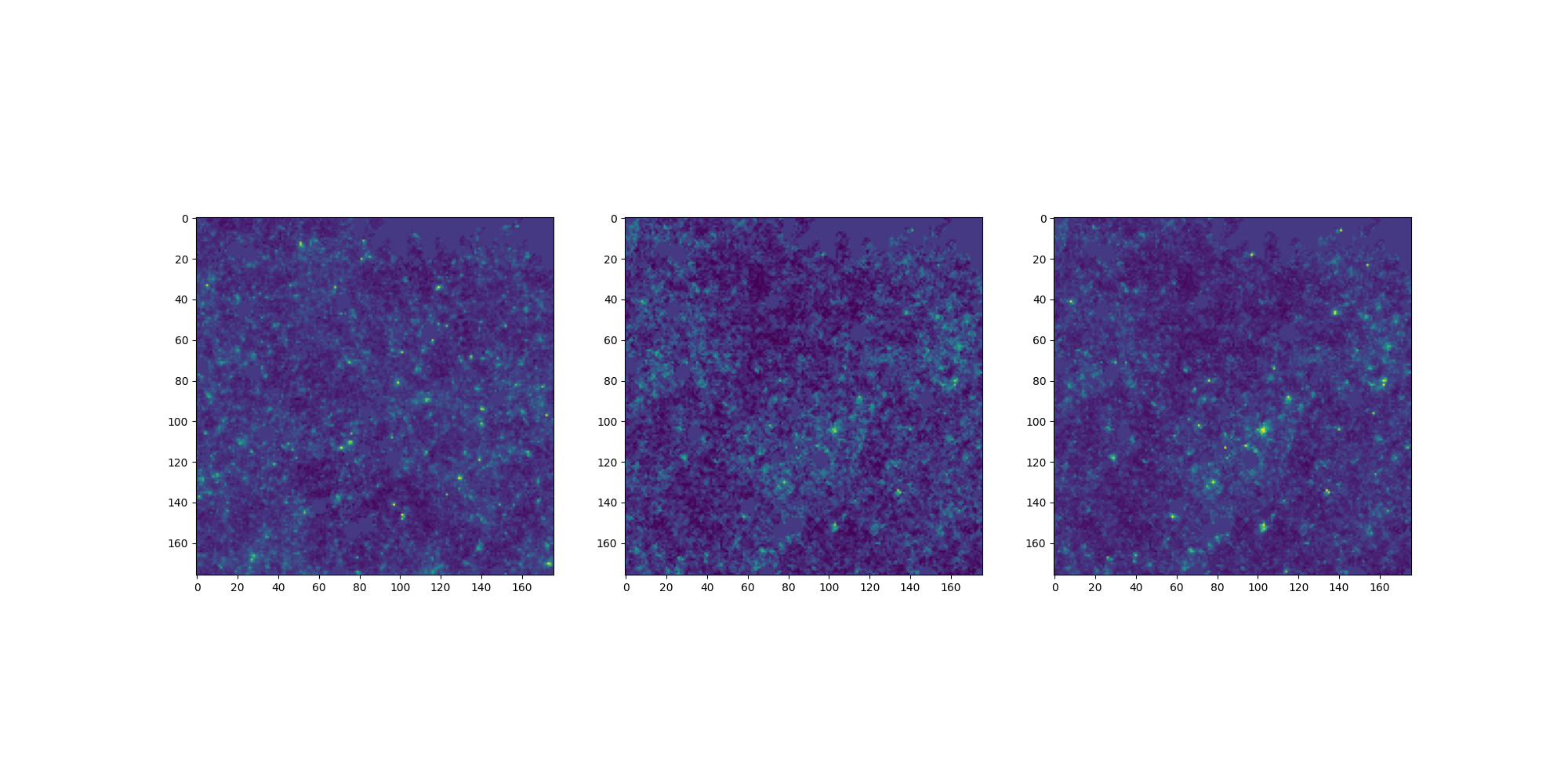
Validating the emulated maps
Power spectrum


LogNormal
Emulated

Challenge simulation
Validating the emulated maps
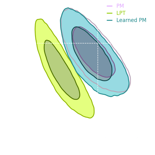
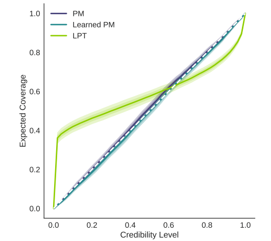
Beyond summary statistics: coverage tests
COT, Cosmostat Journal Club
By Benjamin REMY


