Particle Filter for Identifying and Correcting Phase Transitions in Semi-Coherent GNSS Signals
Brian Breitsch Jade Morton
University of Colorado Boulder
ION GNSS+ 2019
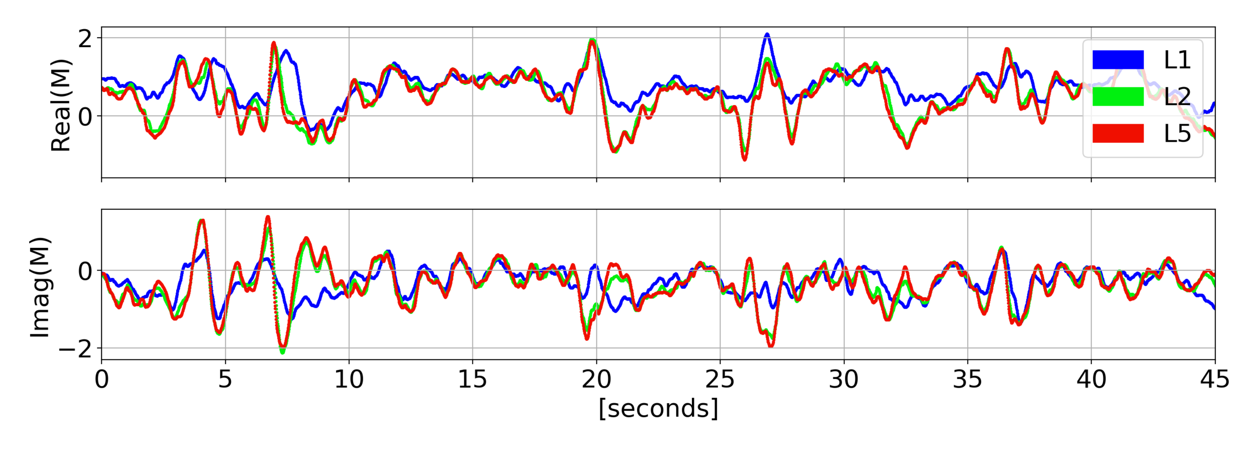
Semi-Coherent Signals:
- random short-delay multipath in the presence of a dominant direct signal
- adverse impact on carrier phase measurement
- particularly prevalent in remote-sensing applications
ionosphere scintillation
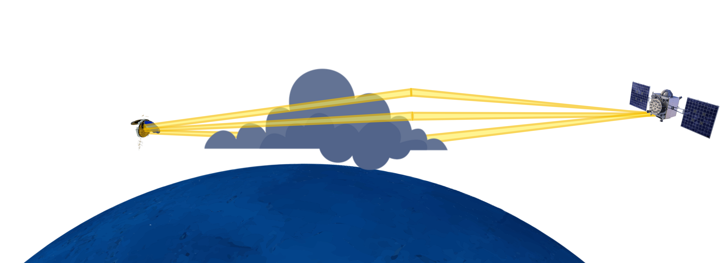
radio occultation / troposphere scintillation
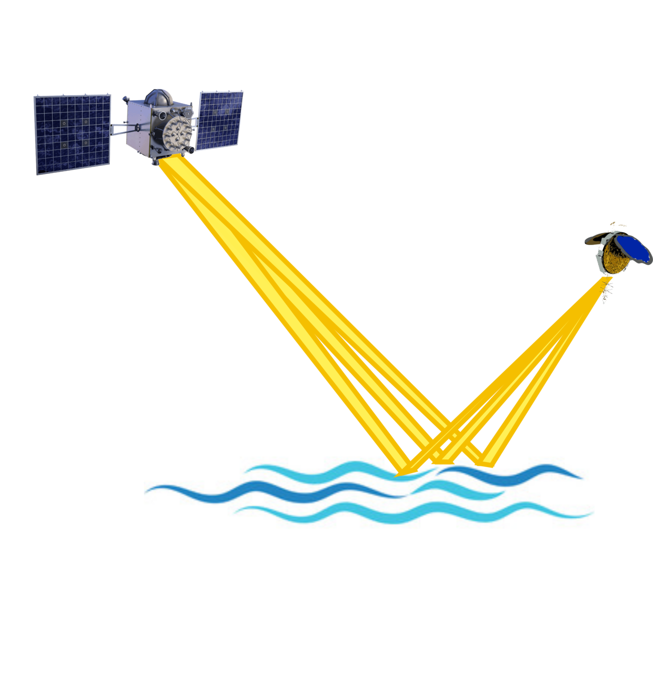
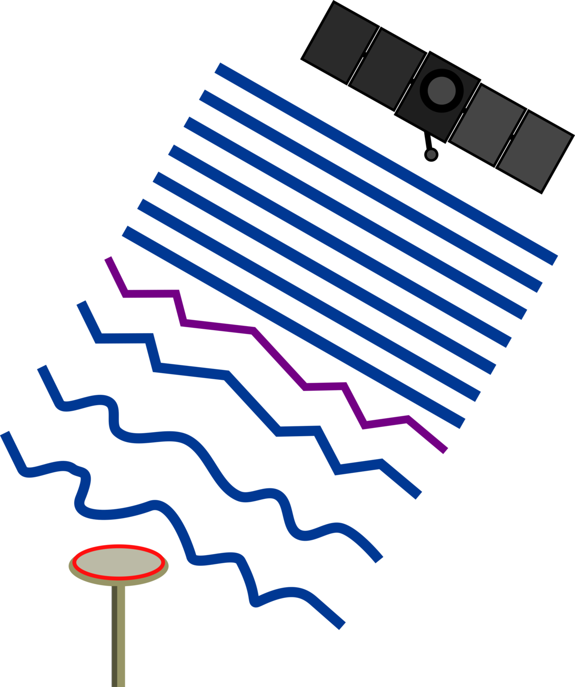
ocean reflection
Motivation: Semi-Coherent Examples
Problem: Phase Transitions
Solution: Particle Filter Algorithm
Background: Signal Model
Semi-Coherent Signals:
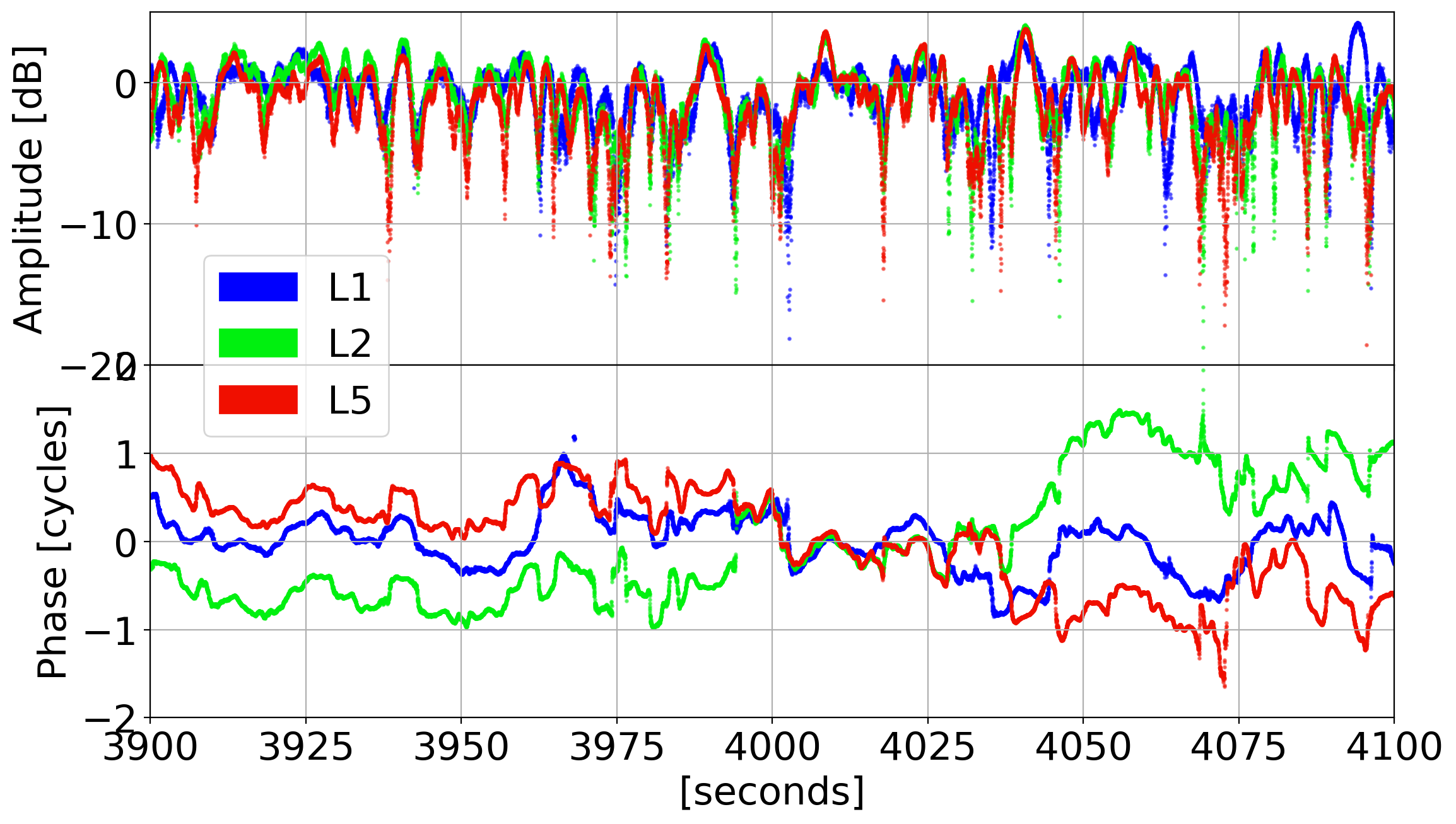
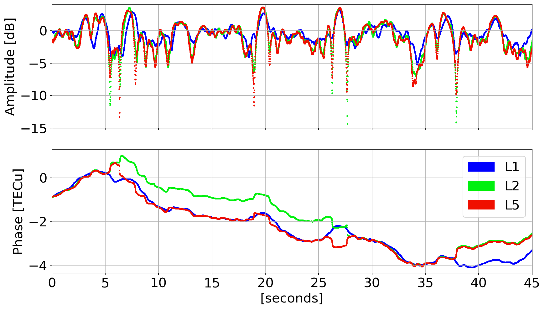
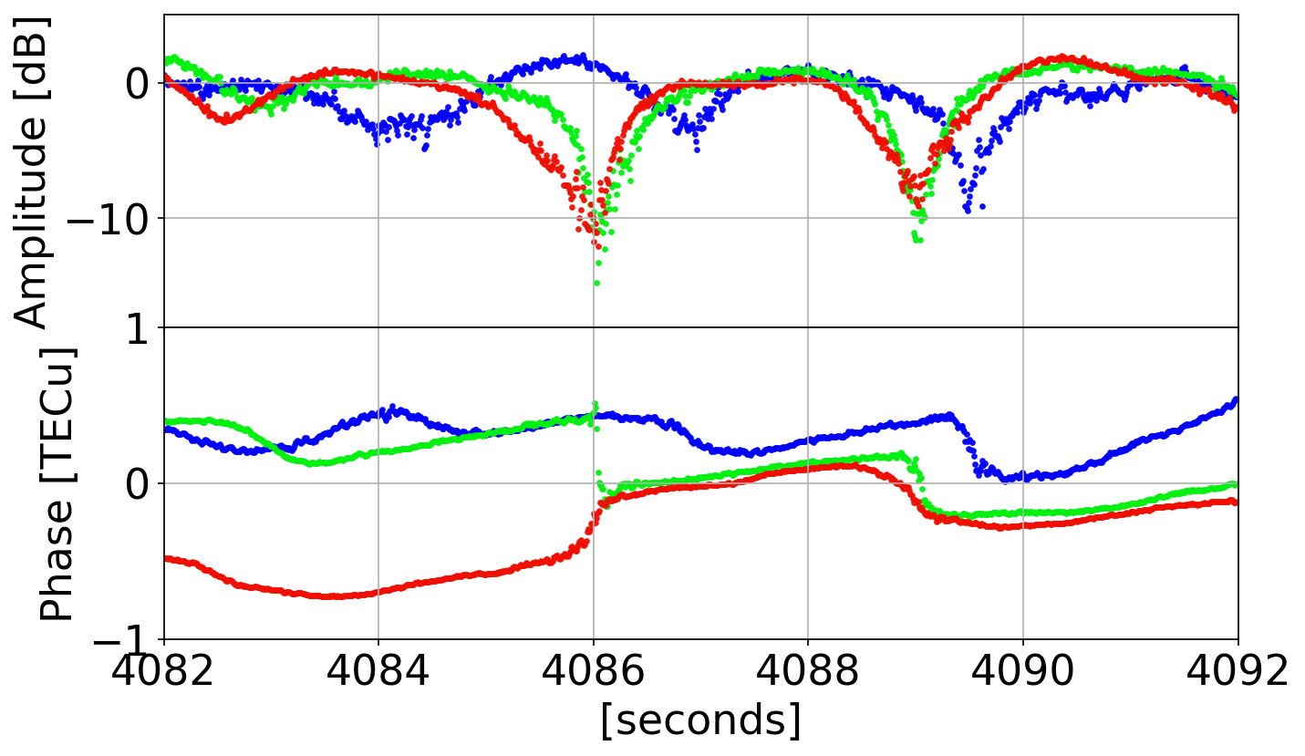
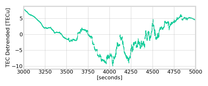
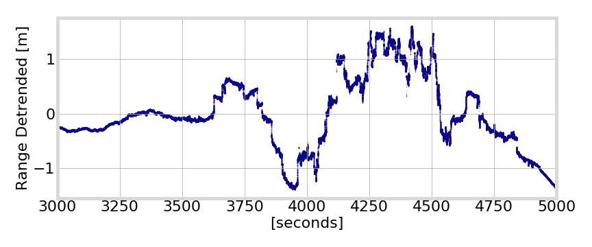
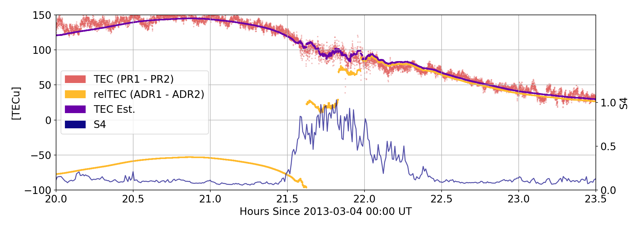
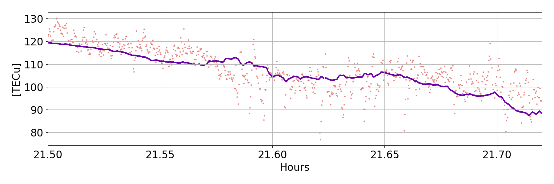
Ionosphere Scintillation (Ascension Island)
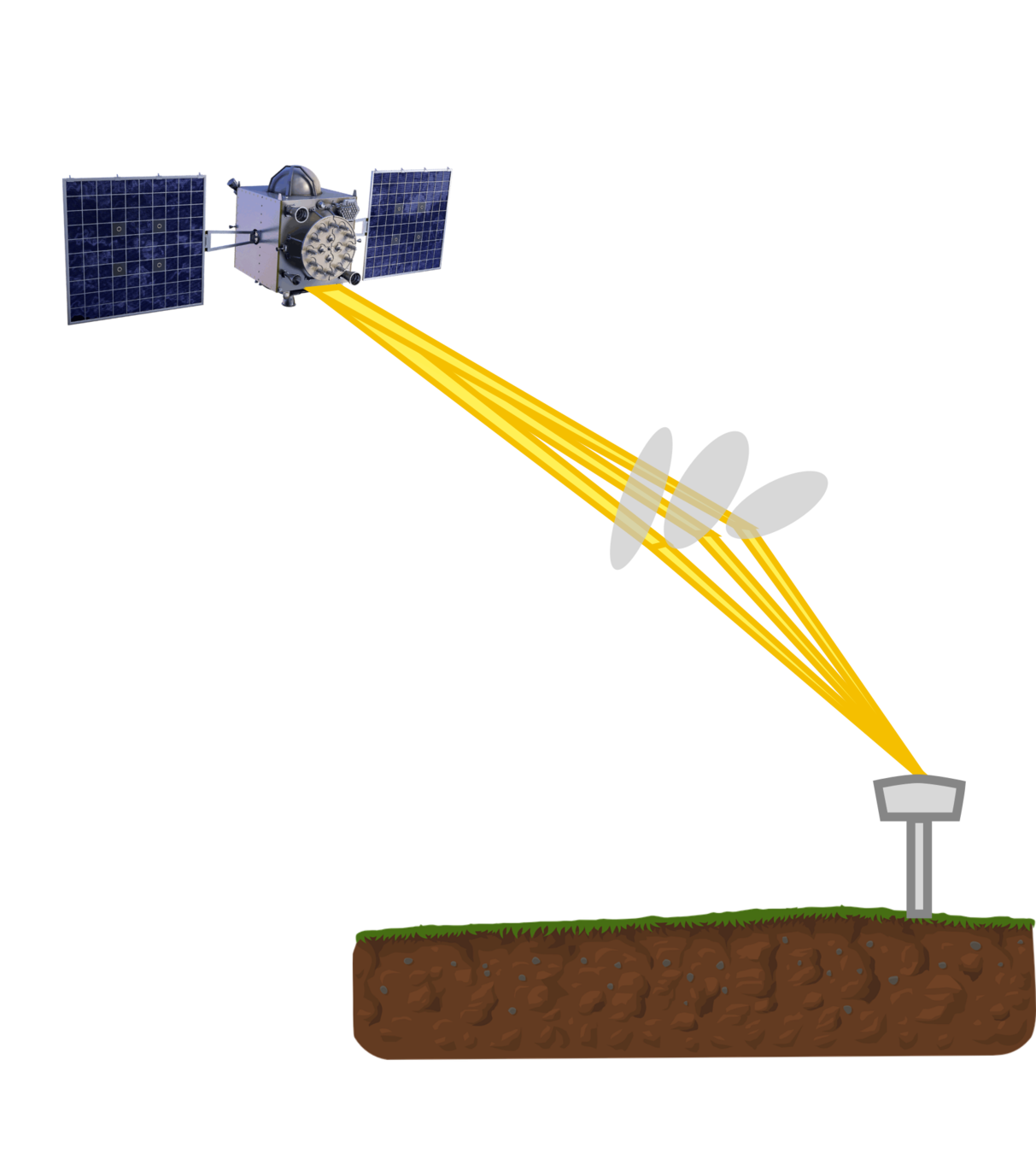
Semi-Coherent Signals:
Troposphere Scintillation (Hawaii)

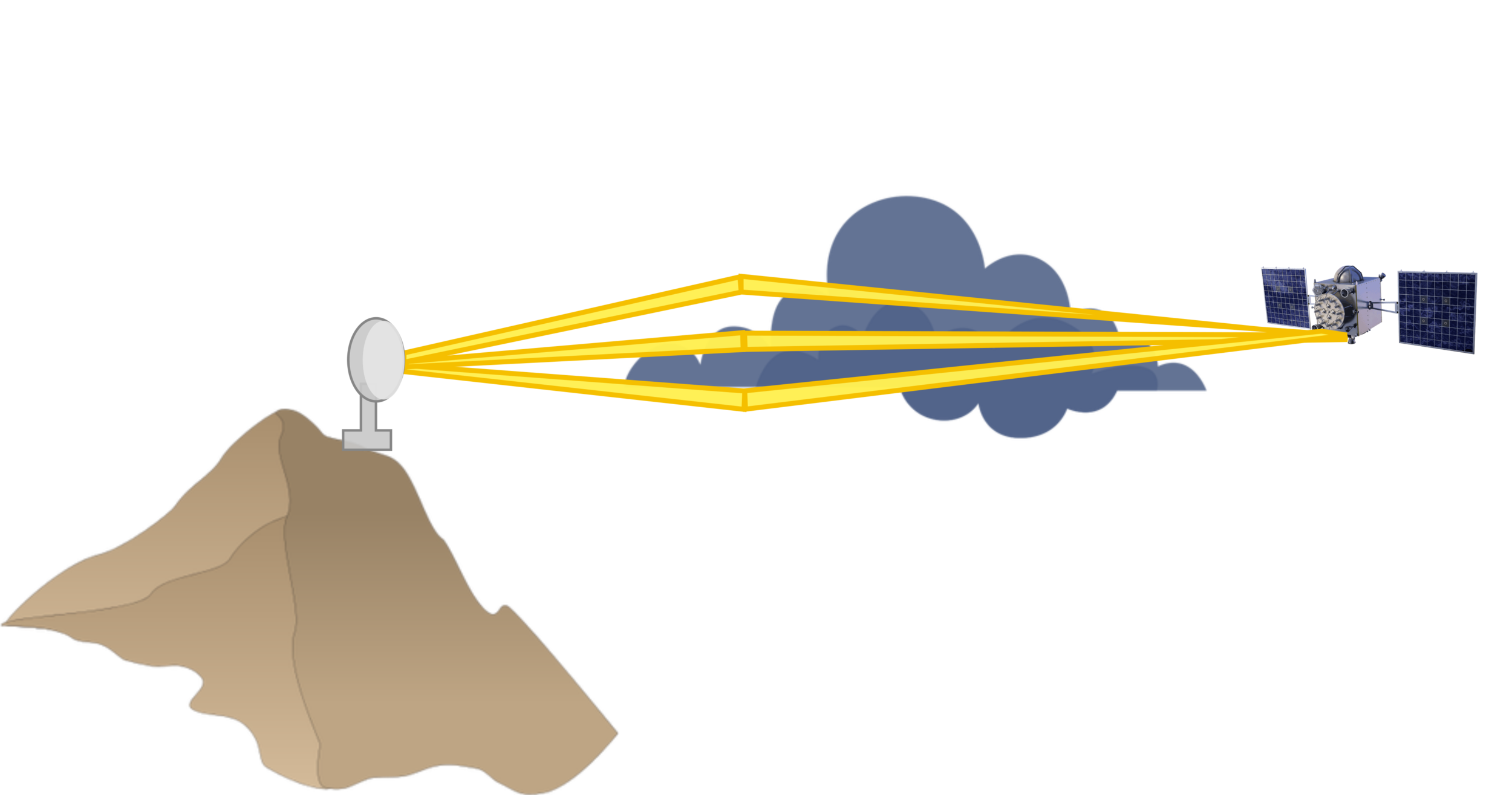
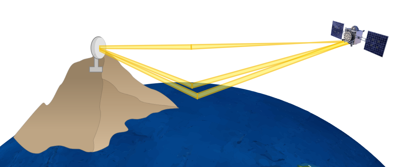
Semi-Coherent Signals:
Ocean Reflection (Hawaii)
GPS L1 (PRN 30)
Motivation: Semi-Coherent Examples
Problem: Phase Transitions
Solution: Particle Filter Algorithm
Background: Models
Signal Model

REFRACTIVE IONOSPHERE EFFECT
MULTIPATH PHASE EFFECT
FREQUENCY INDEPENDENT EFFECTS
A_k\exp(i\phi_k)
\frac{\lambda_k}{2\pi} \phi_k= G + \alpha_k T + \frac{\lambda_k}{2\pi}\tilde{\phi}_k
M_k = \tilde{A}_k\exp(i\tilde{\phi}_k)
phase model
baseband signal
multipath model
A = \tilde{A}
Assume normalized signal power; amplitude measurements are direct measurements of \(\tilde{A}\)
State-Space Model
\mathbf{x} = \begin{bmatrix} G \\ T \\ \tilde{\phi}_{L1} \\ \tilde{\phi}_{L2} \\ \tilde{\phi}_{L5} \\ \tilde{A}_{L1} \\ \tilde{A}_{L2} \\ \tilde{A}_{L5} \end{bmatrix}
state
% \mathbf{y} = \begin{bmatrix} \phi_{L1} \\ \phi_{L2} \\ \phi_{L5} \end{bmatrix} = H \mathbf{x}
\mathbf{y} = H\mathbf{x} = \begin{bmatrix} \phi_{L1} \\ \phi_{L2} \\ \phi_{L5} \\ A_{L1} \\ A_{L2} \\ A_{L5} \end{bmatrix} + \mathbf{\epsilon}
measurements
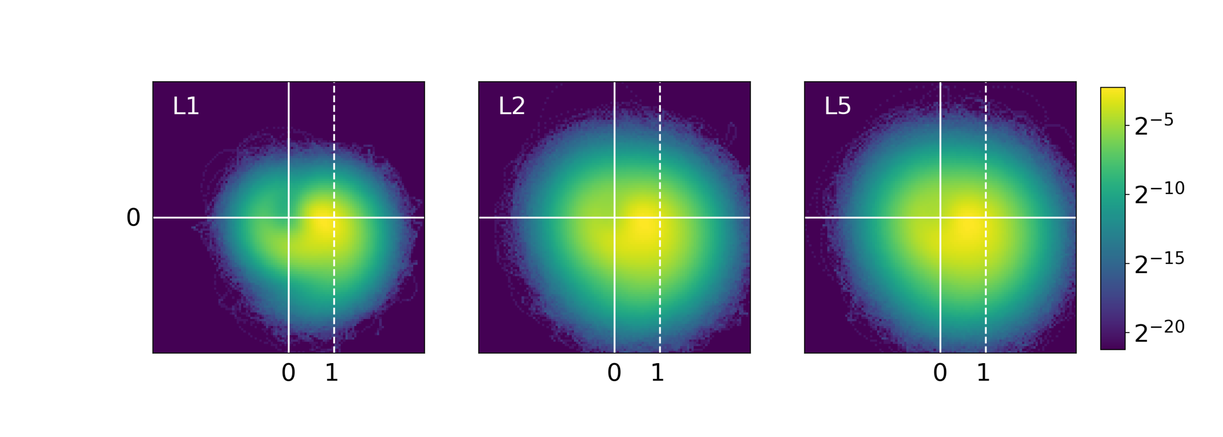
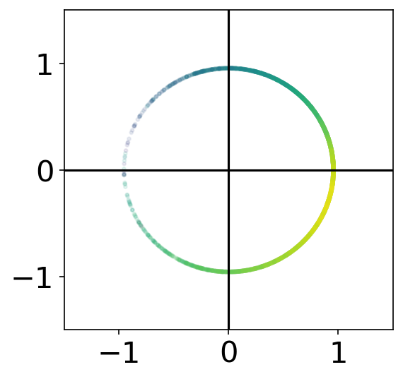
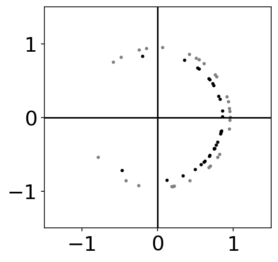
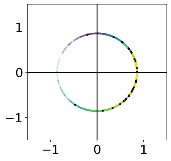
Multipath Model
M_k = \tilde{A}_k\exp(i\tilde{\phi}_k)
coherent multipath
weak scintillation
strong scintillation
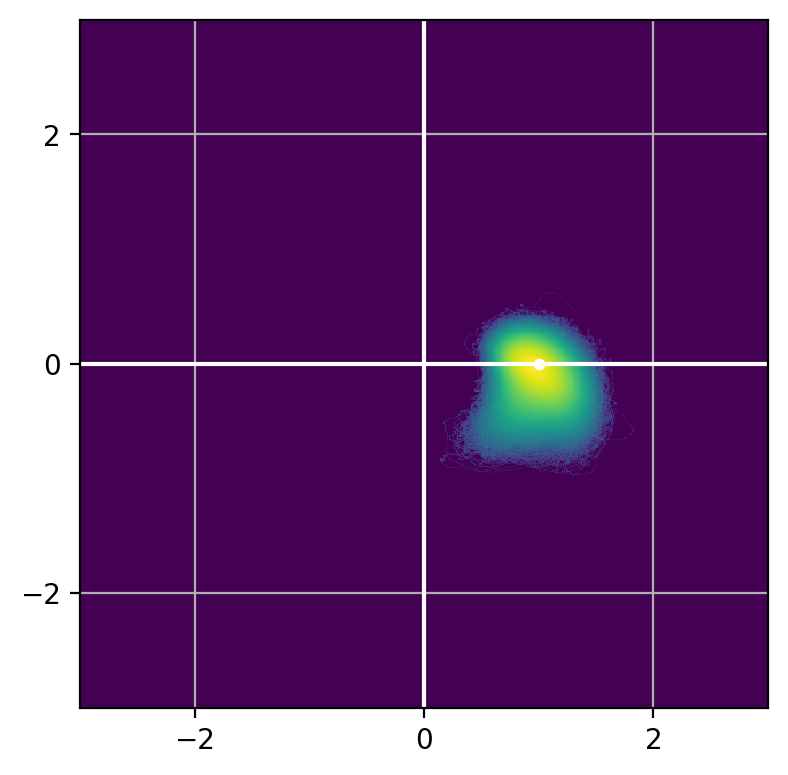
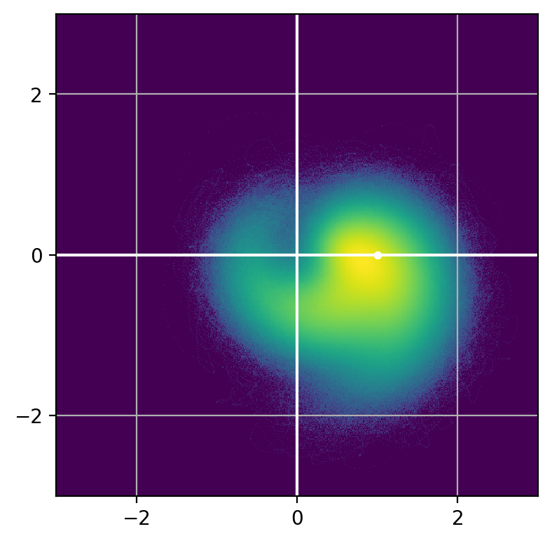
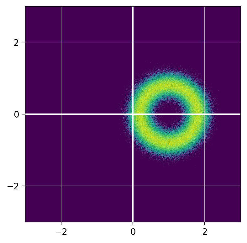
Whether deterministic or stochastic, we can model \(M\)
Re
Im
Scintillation Simulator
- multi-frequency scintillation simulator using physics-based phase screen model
We use this example to test the particle filter algorithm
Jiao, Y., Xu, D., Rino, C. L., Morton, Y. T., & Carrano, C. S. (2018). A Multifrequency GPS Signal Strong Equatorial Ionospheric Scintillation Simulator: Algorithm, Performance, and Characterization. IEEE Transactions on Aerospace and Electronic Systems, 54(4), 1947-1965.
Motivation: Semi-Coherent Examples
Problem: Phase Transitions
Solution: Particle Filter Algorithm
Background: Signal Model
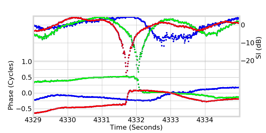
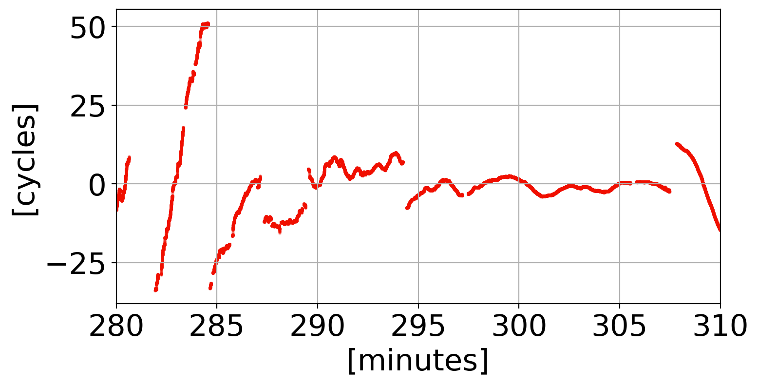
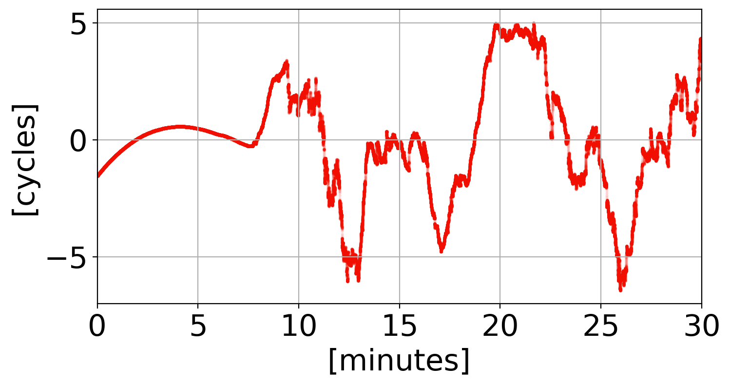
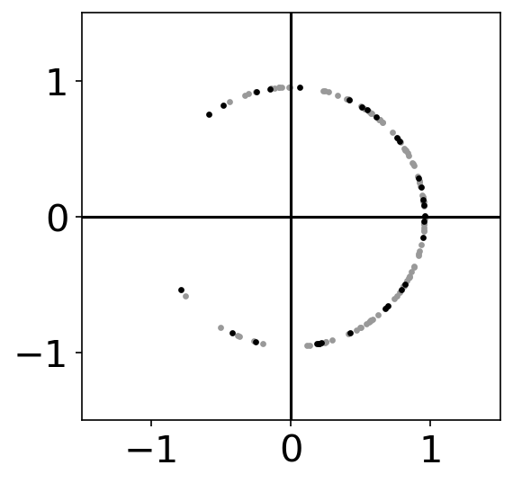
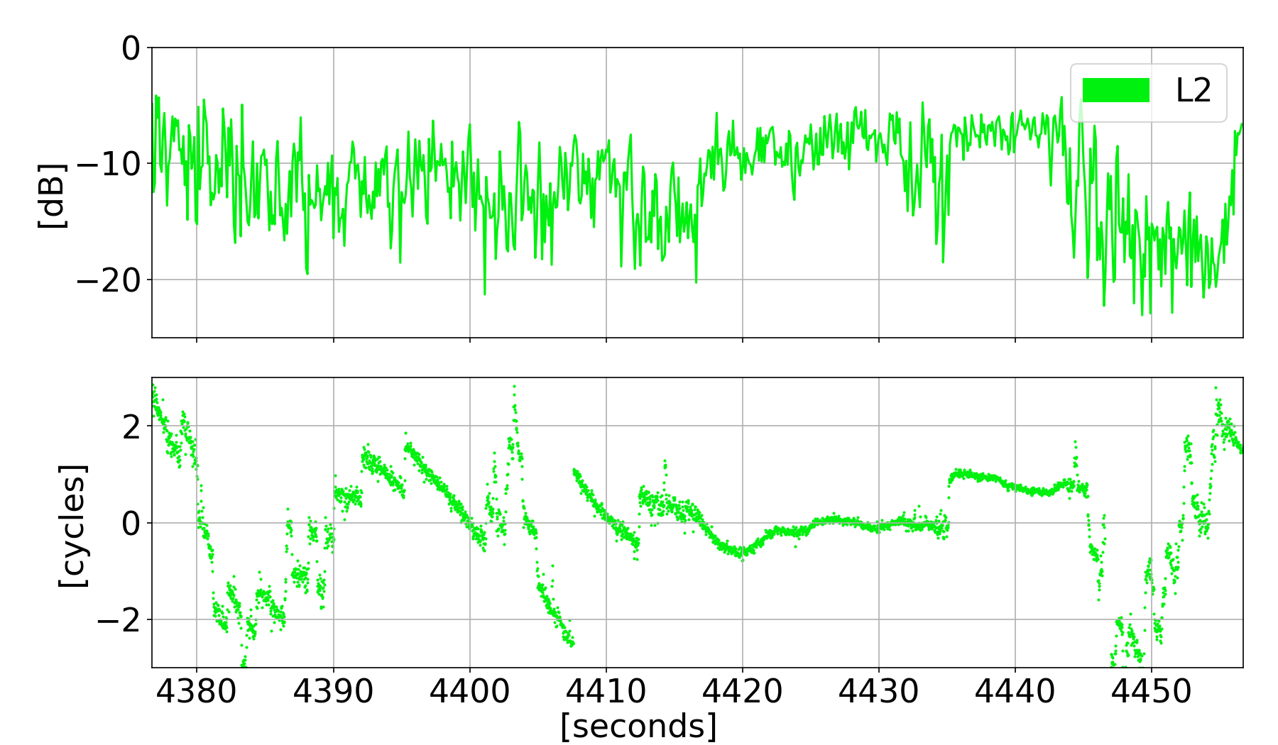
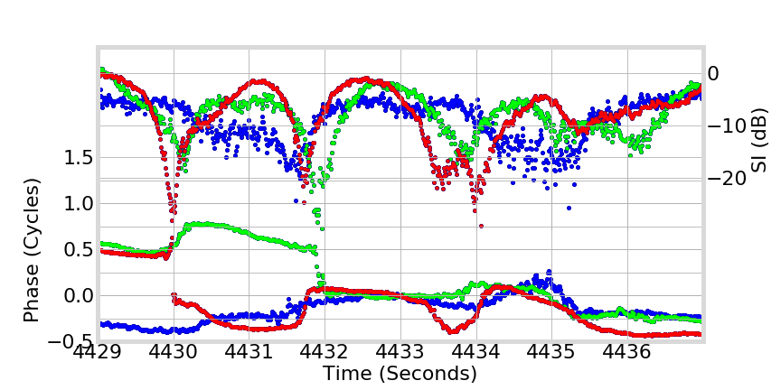
Phase Transitions
not instantaneous!
difficult to discriminate occurrence!
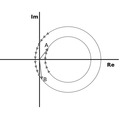
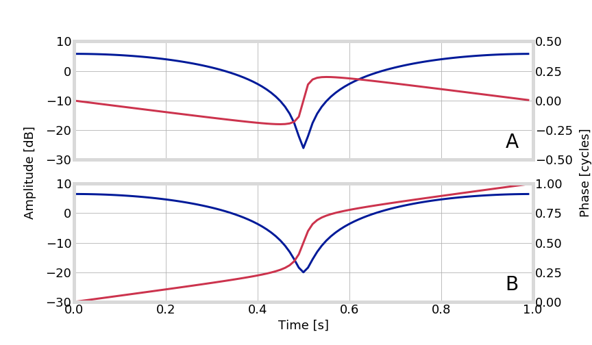
- singularity at origin causes phase bifurcation
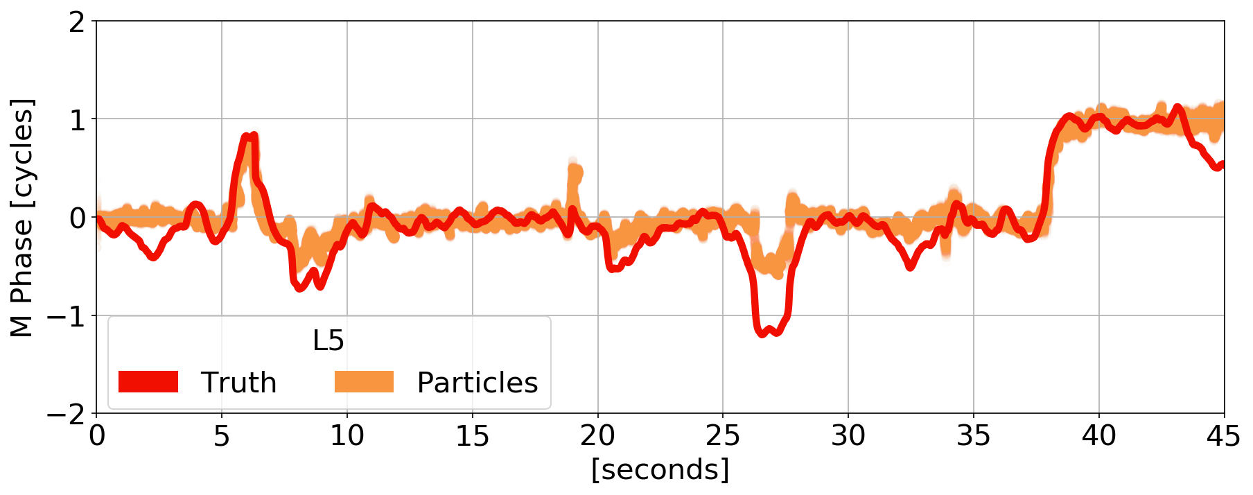
L5
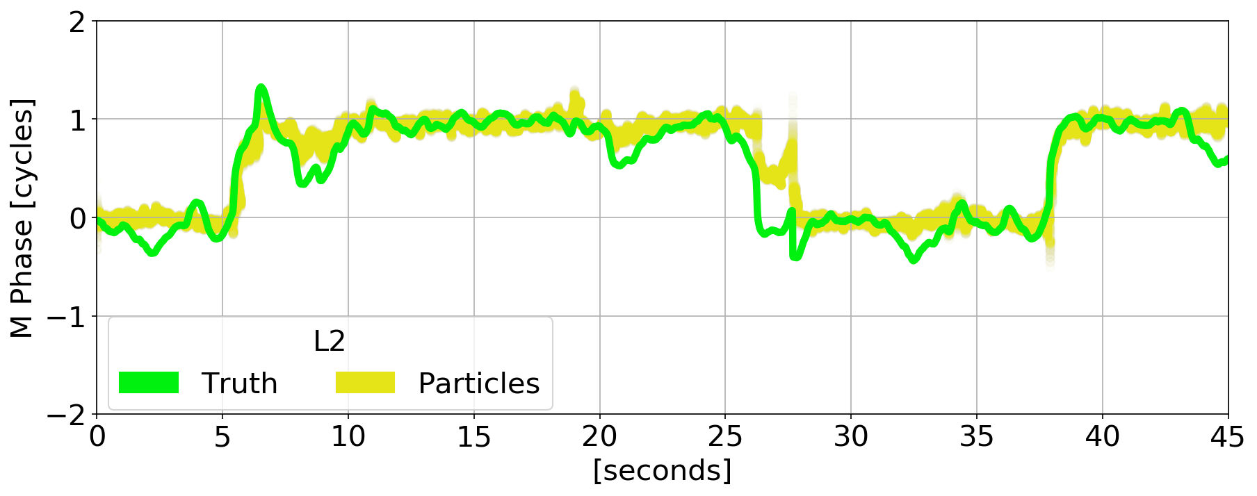
L2
L1
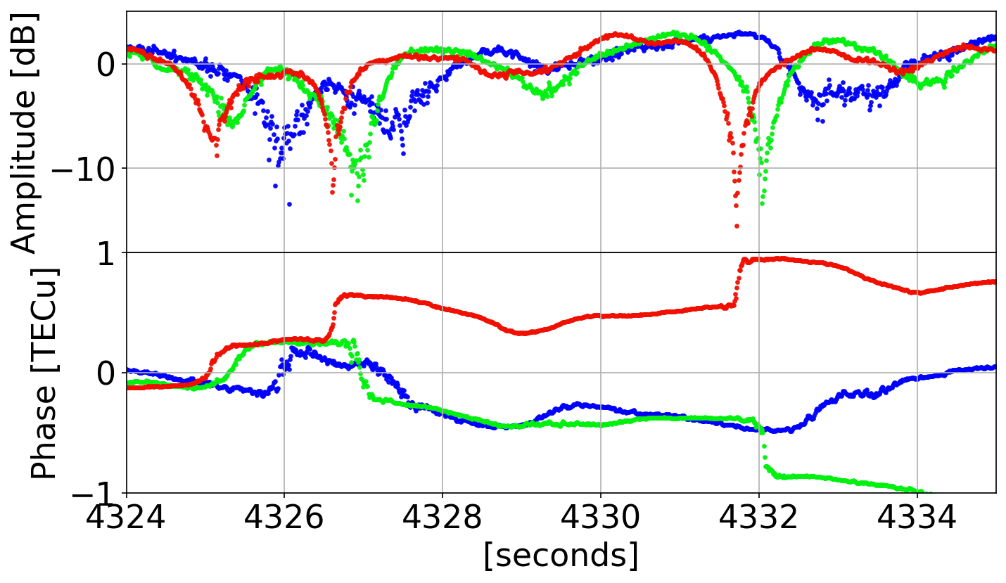
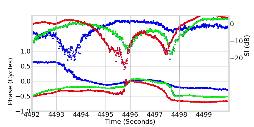
Phase Transitions
Examples
L5
L2
L1
Phase Transitions
Examples
Phase Transitions
Linear Combinations
\frac{\lambda_k}{2\pi} \phi_k= G - \alpha_k T - \frac{\lambda_k}{2\pi}\tilde{\phi}_k
Ionosphere-Free (IF)
phase transitions cause correlated errors in state \(G\) and \(T\) estimates
Geometry-Free (GF)
difficult to discriminate state and multipath dynamics
Cycle Slips vs Phase Transitions
- caused by propagation environment (multipath)
- not instantaneous
- usually an artifact of receiver processing
- instantaneous
Addressing phase transitions in semi-coherent signals requires a special approach that incorporates high-rate signal phase and amplitude measurements along with along with robust models of random multipath
generally easier to correct
difficult to even see
Motivation: Semi-Coherent Examples
Problem: Phase Transitions
Solution: (Particle Filter Algorithm)
Background: Signal Model
Why Particle Filter?
- Bayesian, multi-modal
- sequential
- good at dealing with non-linearity
M_k = \tilde{A}_k\exp(i\tilde{\phi}_k)
Sample \(N_p\) states from \(q_1(\mathbf{x}_{1})\)
Compute weights \(w(\mathbf{x}_{1:n}) \propto p(\mathbf{M}) \)
\(\mathbf{M}_n\)
Propagate to time \(n+1\)
Resample from \(q_{n}(\mathbf{x}_{1:n})\)
\(w(\mathbf{x}_n)\)

Particle Filter Details
Posterior Target Distribution
Ideal Measurement Assumption
Initial Proposal Distribution
q_1(\mathbf{x}_{1}) \propto \mathcal{N}(G_1; \mu_{G_1}, 0.05) \mathcal{N}(T_1; \mu_{T_1}, 0.1) \delta(\mathbf{y}_1 - H\mathbf{x}_1)
p(\mathbf{x}_{1:n} | \mathbf{y}_{1:n}) \propto p(\mathbf{y}_{1:n} | \mathbf{x}_{1:n})p(\mathbf{x}_{1:n})
Subsequent Proposal Distribution
q_n(\mathbf{x}_{1:n}) \propto \mathcal{N}(G_n; G_{n-1}, \sigma_{G_n}^2)\mathcal{N}(T_n; T_{n-1}, \sigma_{T_n}^2) \delta(\mathbf{y}_n - H\mathbf{x}_n)
p(\mathbf{y}_{1:n} | \mathbf{x}_{1:n}) = \delta(\mathbf{y}_{1:n} - H\mathbf{x}_{1:n})
- reduces problem dimensionality
- measurement noise can be partially absorbed into \(\mathbf{M}\) model
Weights
w(\mathbf{x}_{1:n}) \propto p(\mathbf{M}_n|\mathbf{M}_{n-1})
Other Details
- systematic resampling
- 5000 particles
Multipath Dynamics Model
How can we define \(p(\mathbf{M}_{(1:n)})\)?
-
highly-correlated non-linear random process
- we approximate locally-normal correlated random process with state-dependent covariance
p(\mathbf{M}_n|\mathbf{M}_{n-1})\sim\mathcal{N}(\mathbf{M}_{n-1}, \Sigma(\mathbf{M}_{n-1})) p_0(M_n)
p_0(M_n)
Results...
This was not a resounding success.
But we still can learn a lot.
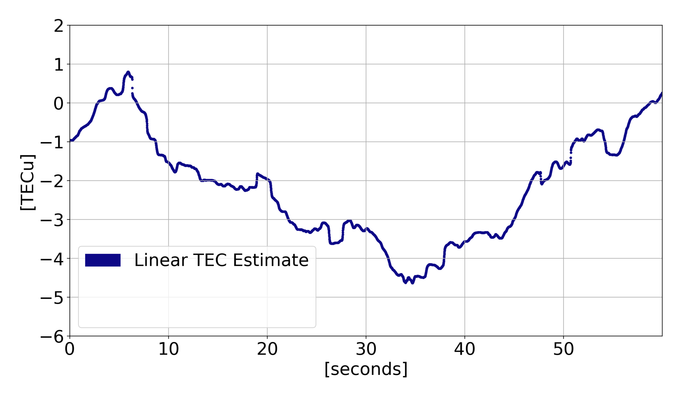
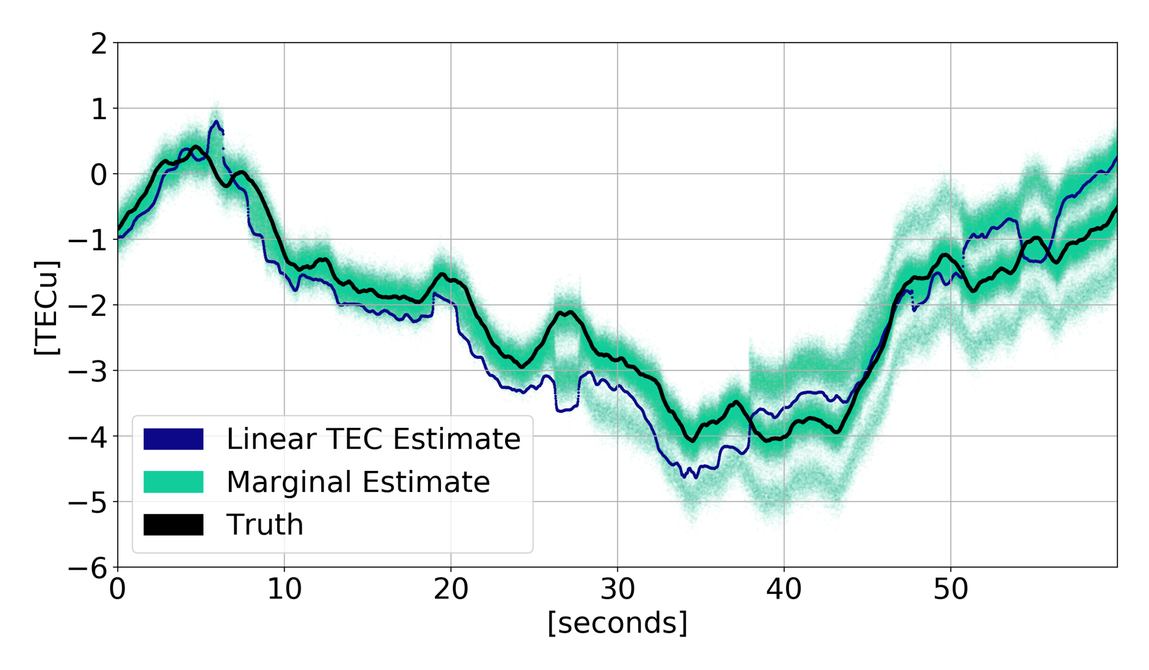
Estimation Results
\(\tilde{\phi}\) Errors
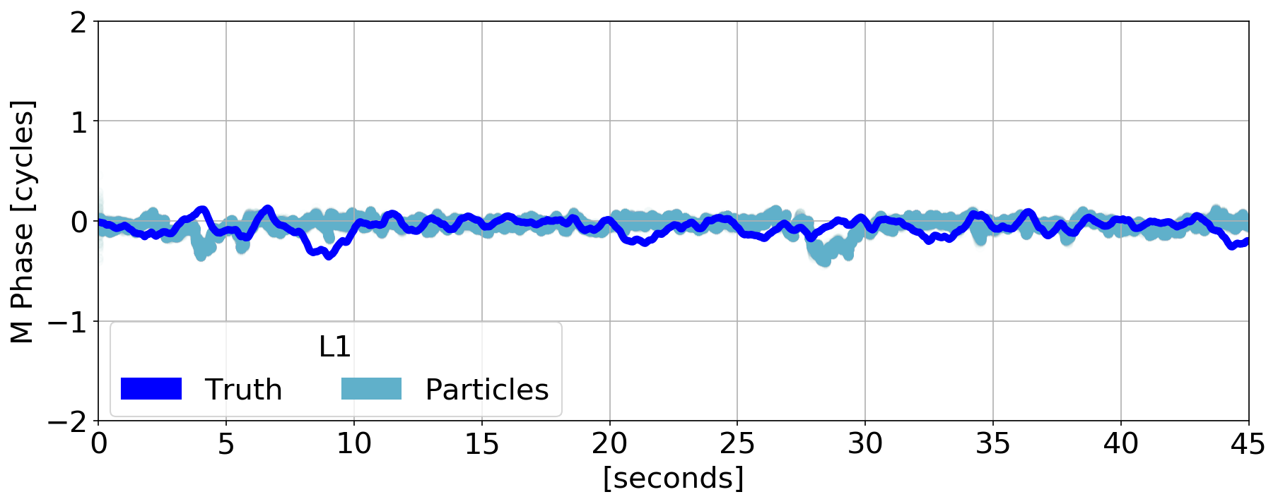
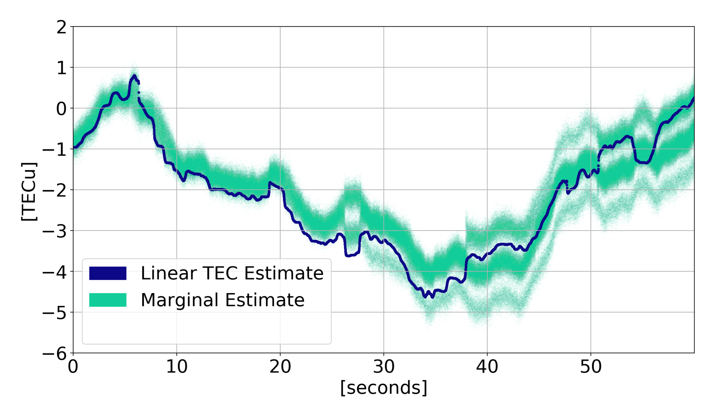
Estimation Results
\(\tilde{\phi}\) Errors
Estimation Results
\(G\) and \(T\) Errors
- Avoids jumps and biases due to phase transitions
- Filters some diffraction fluctuations
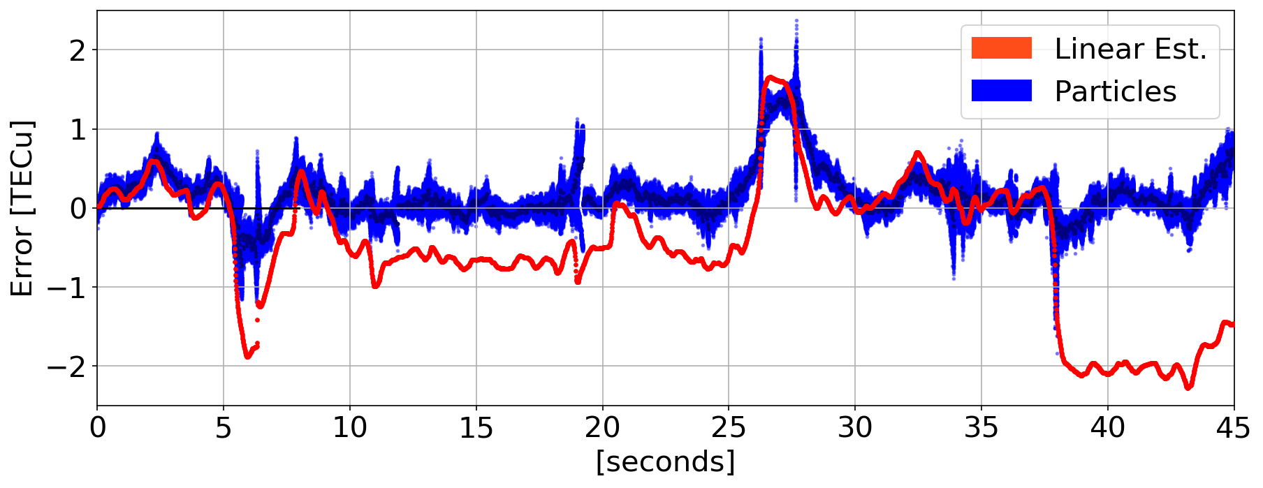
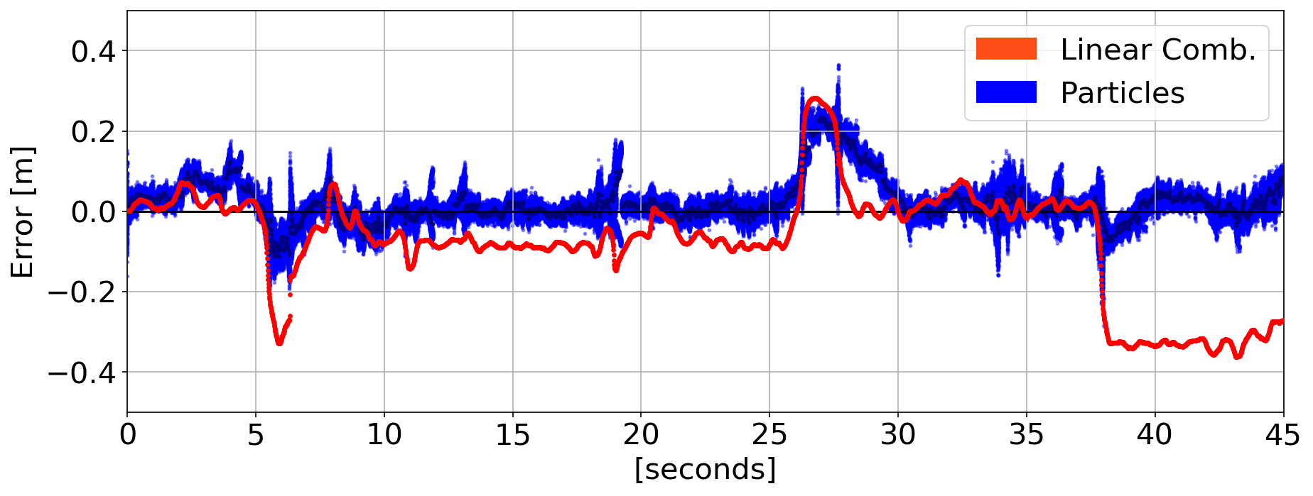
\(G\)
\(T\)
Particle Filter Summary
How well did this work?
The Good
The Bad
- estimates phase transitions
- marginal bifurcation
- reduced errors in \(G\) and \(T\) estimates
- insufficient spread in state estimate
- particle filter degeneracy
- some large dynamics in \(G\) and \(T\)
Key Points
Motivation:
Phase transitions cause large errors in connected phase from semi-coherent signals
Even with multi-frequency information, discriminating state and multipath dynamics is challenging/ambiguous
Particle Filter:
Not sufficient for separating multipath from other state dynamics
Next Steps:
We will try moving-window Bayesian estimation approaches
Acknowledgements
Contact
Brian Breitsch
brianbreitsch@colorado.edu
Spire
Carolyn J Roesler
Rong Yang
Steve Taylor and Harrison Bourne
- LEO ocean reflectometry data
- Help with Spire data
- Help with mountaintop RO data
- GNSS data collection
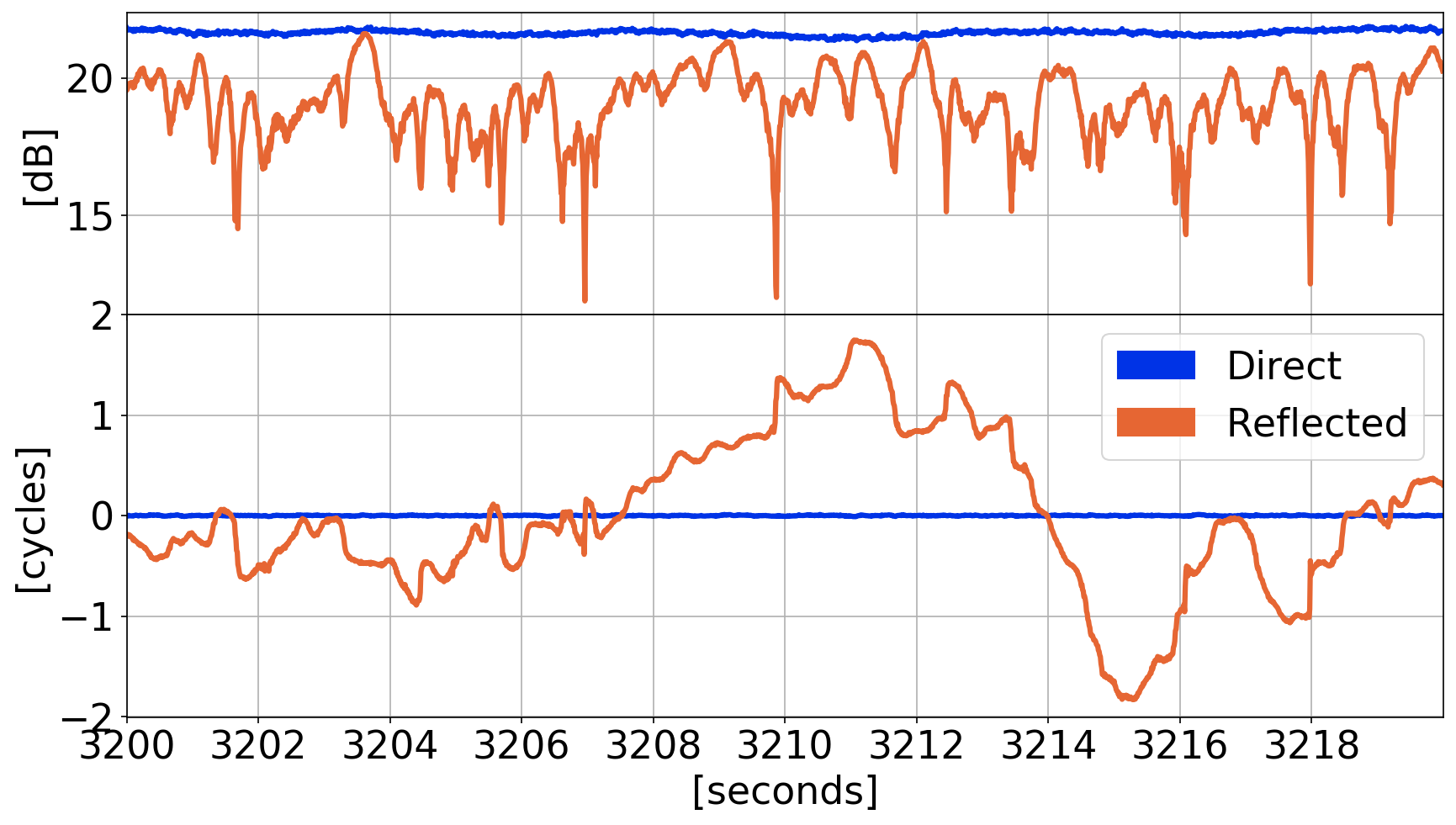
Semi-Coherent Signals:
Ocean Reflection (Spire satellite)
\(\text{reflected} - \text{direct}\)
L5
L2
L1
Phase Transitions
Examples
Why Particle Filter?
- Bayesian
- sequential
- good at dealing with non-linearity
M_k = \tilde{A}_k\exp(i\tilde{\phi}_k)
L5
L2
L1
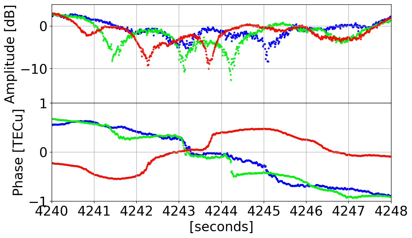
Phase Transitions
Ascension Island


L5
L2
L1
Phase Transitions
Ascension Island
Phase Transitions
Attempted removal in real scintillation data (Hong Kong, Septentrio ground antenna)
phase transitions
Particle Filter Details
Perfect Measurement Assumption
If we assume no phase measurement noise, then:
p(\mathbf{y}|\mathbf{x}) = \delta(\mathbf{y}_\Phi - H_\Phi\mathbf{x}) p(\mathbf{y}_A | \mathbf{x}_A)
and
p(\mathbf{x}|\mathbf{y}) = \frac{\delta(\mathbf{y} - H\mathbf{x}) p(\mathbf{x})}{p(\mathbf{y})}
i.e. find the most likely state sequence that satisfies our measurements.
prior probability of state sequence
this is the hard part
not straightforward
Particle Filter to Identify and Correct for Phase Transitions in Semi-Coherent GNSS Signals
By Brian Breitsch
Particle Filter to Identify and Correct for Phase Transitions in Semi-Coherent GNSS Signals
ION GNSS meeting 2019


