Analysis of Real and Simulated Carrier Phase Residuals
Brian Breitsch\(^1\)
Jade Morton\(^1\)
Charles Rino \(^2\)
In the Geometry-Ionosphere-Free Combination
URSI NRSM 2018
1. University of Colorado Boulder
2. Boston College
Background and Motivation
Geometry-Ionosphere-Free Combination
Derivation and Examples
Analysis and Comparison
Description of IPE Method
Comparison of Real and Simulated GIFC
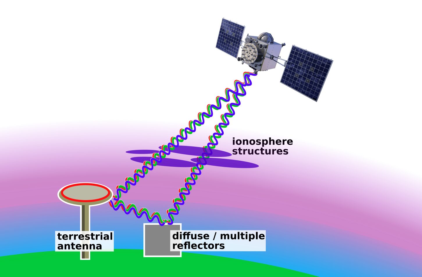
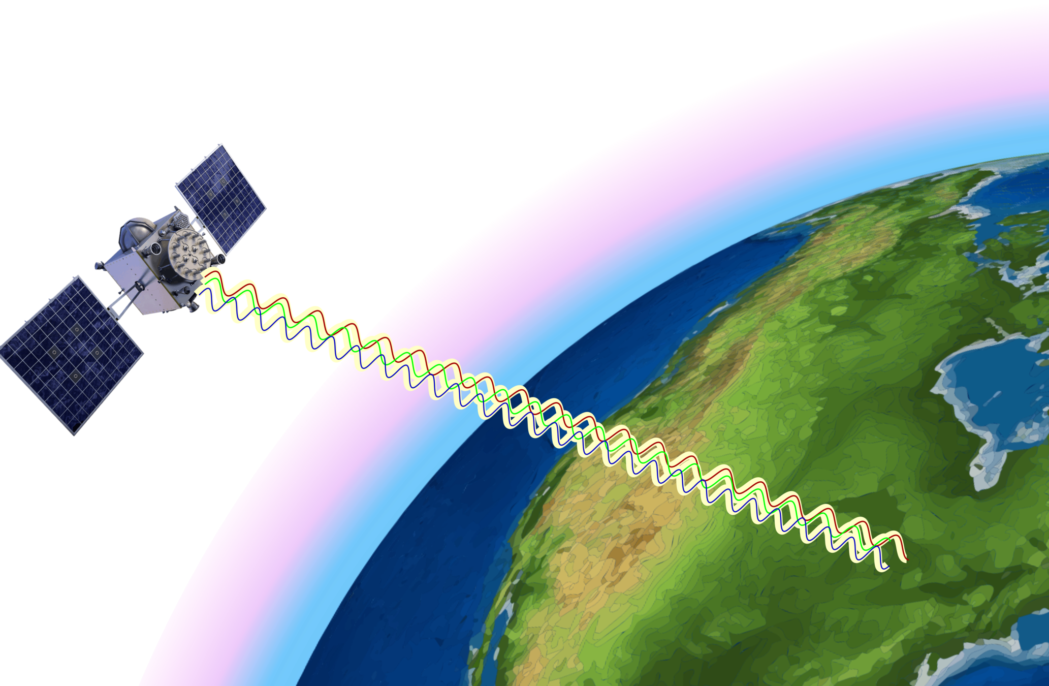
GNSS Carrier Phase
Scintillation
Dual vs Triple-Frequency GPS
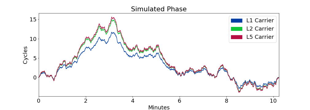
Phase Simulation During Scintillation
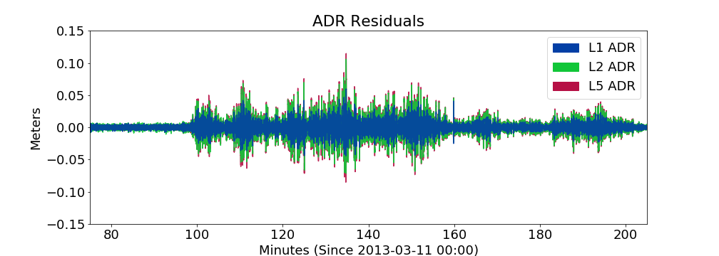
SI, S4, detrended phases and phase combinations
Qualitative look at triple-frequency scint. examples
Carrier Phase Measurement

\Phi_i = r + c\Delta t + T + I_i + \lambda_i N_i + H_i + S_i + \epsilon_i
BIASES
IONOSPHERE RANGE ERROR
CARRIER AMBIGUITY
SYSTEMATIC ERRORS / MULTIPATH
FREQUENCY INDEPENDENT EFFECTS
STOCHASTIC ERRORS
I_i \approx -\frac{\kappa}{f_i^2} \text{TEC}
scintillation
Scintillation Effect
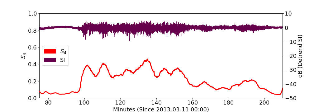
fairly weak
S_4 < 0.5
6th-order Butterworth Highpass with 0.1 Hz cutoff
Estimation Using Dual-Frequency GNSS
\text{TEC} = \displaystyle -\frac{\Phi_1 - \Phi_2}{\kappa \left(\frac{1}{f_1^2} - \frac{1}{f_2^2}\right)}
G = \displaystyle \frac{f_1^2 \Phi_1 - f_2^2 \Phi_2}{f_1^2 - f_2^2}
ionosphere-free combination
geometry-free combination
\Phi_i = G + I_i + S_i + \epsilon_i
"geometry" term
\Phi_i = r + c\Delta t + T + I_i + \lambda_i N_i + H_i + S_i + \epsilon_i
we can solve bias terms
scintillation will impact residuals of range and TEC estimates
Multi-Frequency GNSS
- GPS Block IIF / Block III
- Galileo (E1, E5a/b)
- GLONASS-K2
| Signal | Frequency (GHz) |
|---|---|
| L1CA | 1.57542 |
| L2C | 1.2276 |
| L5 | 1.17645 |
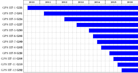
triple-frequency GPS
12 satellites since 2016
(higher-quality signal)
Estimation Using Triple-Frequency GNSS
ionosphere-free combination
geometry-free combination
\Phi_i = G + I_i + S_i + \epsilon_i
\sum_i c_i = 0
\sum_i \frac{c_i}{f_i^2} = 0
\begin{matrix}
\text{Estimate} & c_1 & c_2 & c_3 & \text{noise amp.} \\[.5em]
& & & & \\
& & & & \\
G_\text{L1,L2,L5} & 2.3 & -0.4 & -1.0 & 2.5 \\
& & & & \\
& & & & \\
& & & & \\
\text{TEC}_\text{L1,L2,L5} & 8.3 & -2.9 & -5.4 & 10.3 & \\
\end{matrix}
c_1 \Phi_1 + c_2 \Phi_2 + c_3 \Phi_3
Triple-Frequency GPS Coefficients
Background and Motivation
Geometry-Ionosphere-Free Combination
Derivation and Examples
Analysis and Comparison
Description of IPE Method
Comparison of Real and Simulated GIFC
GNSS Carrier Phase
Scintillation
Dual vs Triple-Frequency GPS
Phase Simulation During Scintillation
SI, S4, detrended phases and phase combinations
Qualitative look at triple-frequency scint. examples
Geometry-Ionosphere-Free Combination
ionosphere-free combination
geometry-free combination
\sum_i c_i = 0
\sum_i \frac{c_i}{f_i^2} = 0
c_1 = \alpha \left( \frac{1}{f_3^2} - \frac{1}{f_2^2} \right)
c_1 \Phi_1 + c_2 \Phi_2 + c_3 \Phi_3
c_3 = \alpha \left( \frac{1}{f_2^2} - \frac{1}{f_1^2} \right)
c_2 = \alpha \left( \frac{1}{f_1^2} - \frac{1}{f_3^2} \right)
Triple-Frequency GIFC Coefficients
\alpha =
arbitrary scaling factor
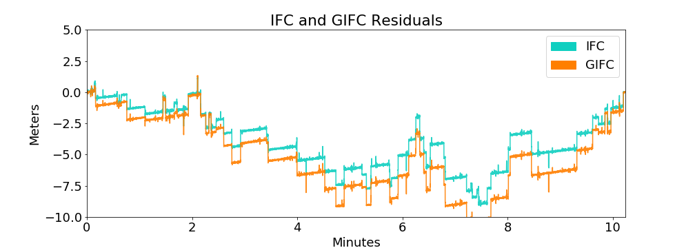
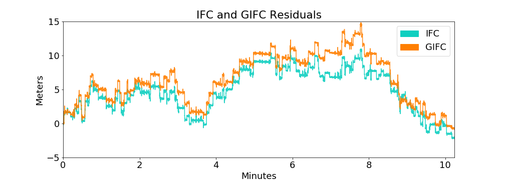
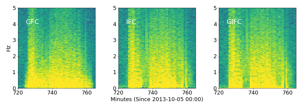
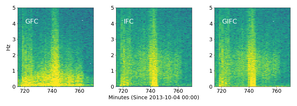
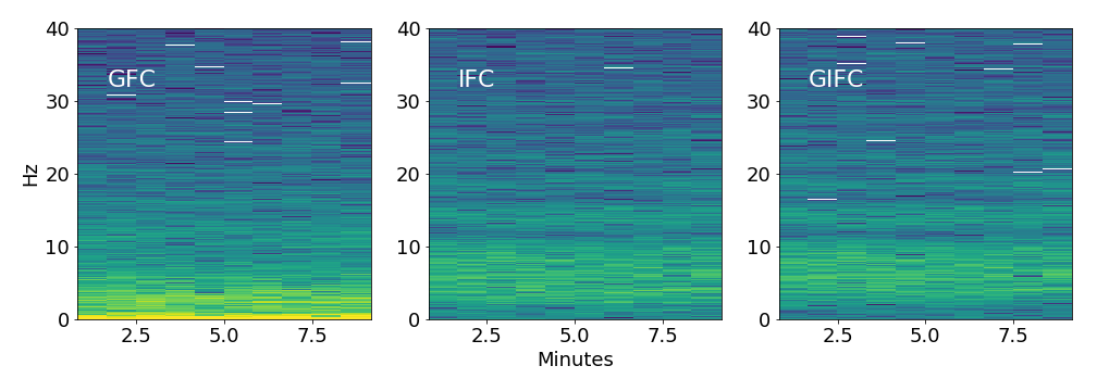
IFC
GFC
GIFC
~TEC
GIFC Examples
PRN 24, Peru
PRN 24, Hong Kong
PRN 25, Peru
PRN 01, Alaska
2013-01-01
2014-05-15
2013-01-01
2014-06-29
GIFC
Sat. Elevation
Coeff. normalized to IFC norm
Background and Motivation
Geometry-Ionosphere-Free Combination
Derivation and Examples
Analysis and Comparison
Description of IPE Method
Comparison of Real and Simulated GIFC
GNSS Carrier Phase
Scintillation
Dual vs Triple-Frequency GPS
Phase Simulation During Scintillation
SI, S4, detrended phases and phase combinations
Qualitative look at triple-frequency scint. examples
Scintillation Simulator
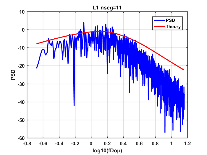
SI Power Spectral Density
from real data
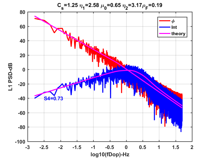
Use Iterative Parameter Estimation (IPE) to resolve structure model params.
Use structure model parameters to derive PSD of complex field at receiver / generate random realization
Background and Motivation
Geometry-Ionosphere-Free Combination
Derivation and Examples
Analysis and Comparison
Description of IPE Method
Comparison of Real and Simulated GIFC
GNSS Carrier Phase
Scintillation
Dual vs Triple-Frequency GPS
Phase Simulation During Scintillation
SI, S4, detrended phases and phase combinations
Qualitative look at triple-frequency scint. examples
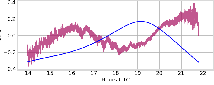
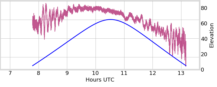
Peru G25 2013-10-30 Example
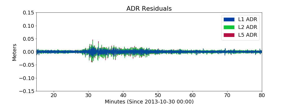
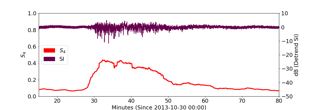
moderately weak
S_4 < 0.5
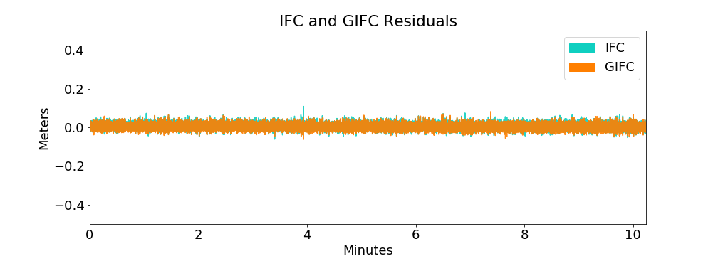
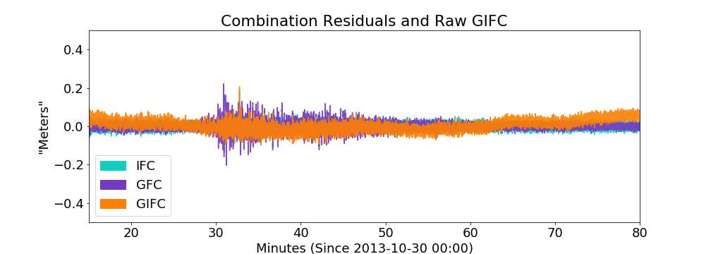
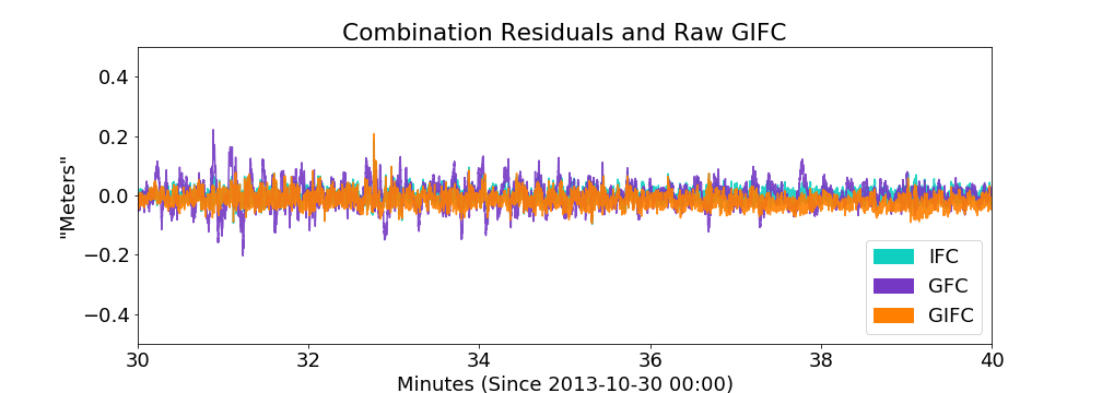
10 minute zoom on real GIFC
10 minute GIFC simulation
model appears to slightly under-represent noise present in real-data GIFC
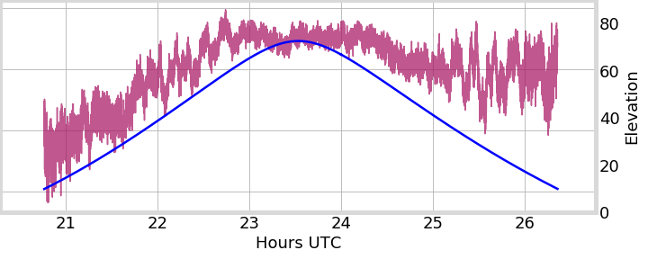
Hong Kong G24 2013-09-24 Example
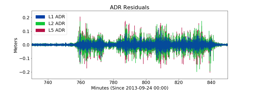
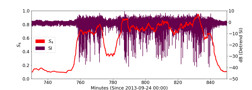
moderately strong
S_4 > 0.8
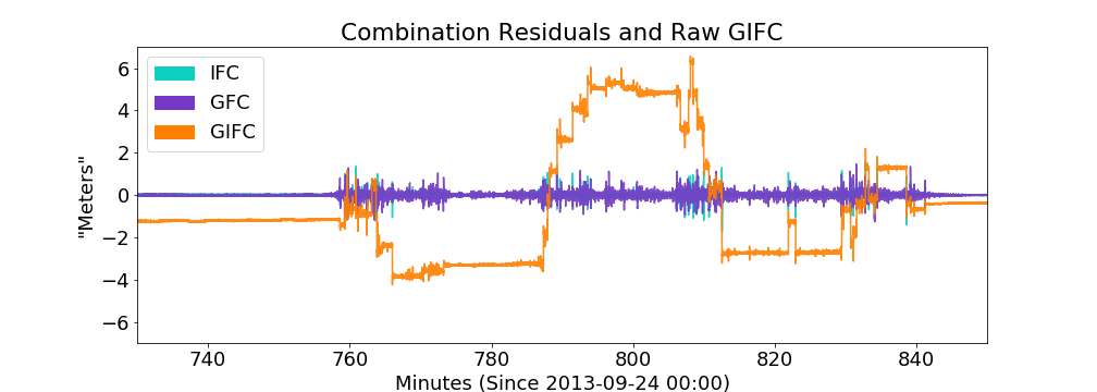
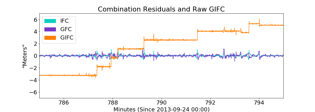
10 minute zoom on real GIFC
10 minute GIFC simulation
more jumps in model realization than actual 10-min data segment
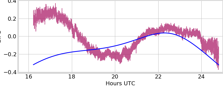
Hong Kong G24 2013-10-05 Example
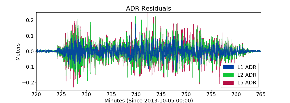
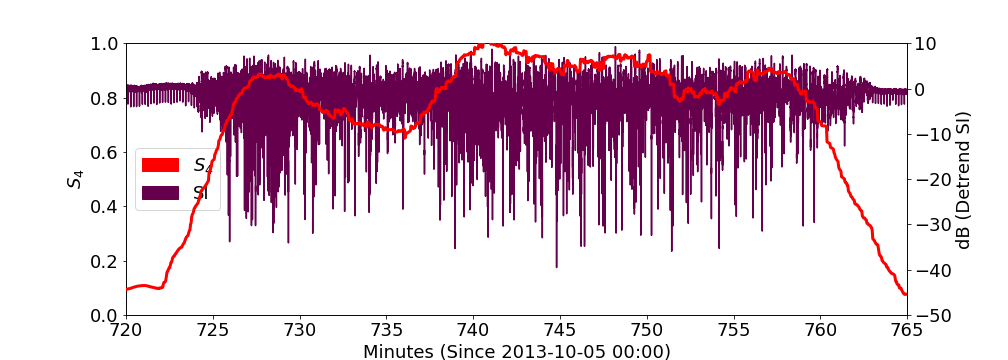
moderately strong
S_4 > 0.8
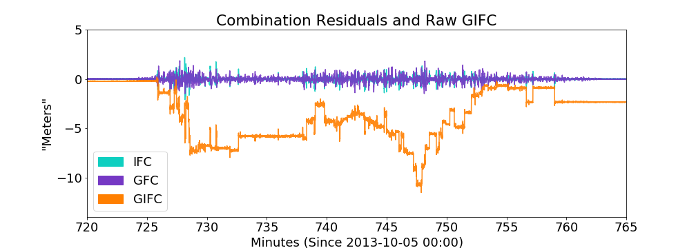
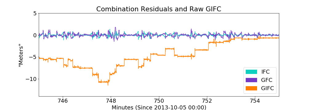
10 minute zoom on real GIFC
10 minute GIFC simulation
again -- more jumps in model realization than real data
Peru G25
Hong Kong G24
Hong Kong G24
10-06
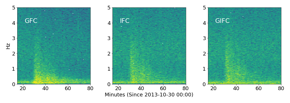
GFC, IFC, GIFC Spectra
Difficulties With IPE and Weak Scintillation
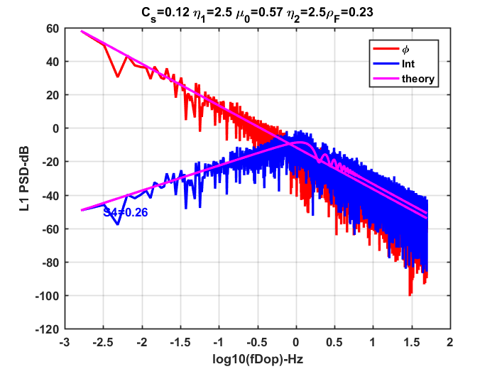
Bad fit?
Bizarre spectrum
Conclusions
- GIFC is an indicator of the presence diffraction effects on GNSS signals
- weak scintillation will not have large effect on GIFC
- although model appears to under-represent small noise increase during weak scintillation
- scintillation model shows many more "jumps" than real data
- need to classify scintillation events
- we can look at more data and start making statistical comparisons
-
IPE fitting for scintillation model is still finicky
- need to explore robustness of current IPE method
Next Steps
Acknowledgements
This research was supported by the Air Force Research Laboratory.
Studying Carrier Phase Residuals Using Triple-Frequency Observations
By Brian Breitsch


