Linear Combinations of GNSS Phase Observables
Brian Breitsch
Advisor: Jade Morton
Committee: Charles Rino, Anton Betten

to Improve and Assess TEC Estimation Precision
Background and Motivation
Linear Estimation of GNSS Parameters
TEC Estimate Error Residuals
Application to Real GPS Data
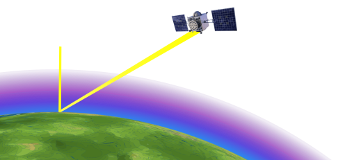
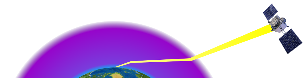
Earth's Ionosphere
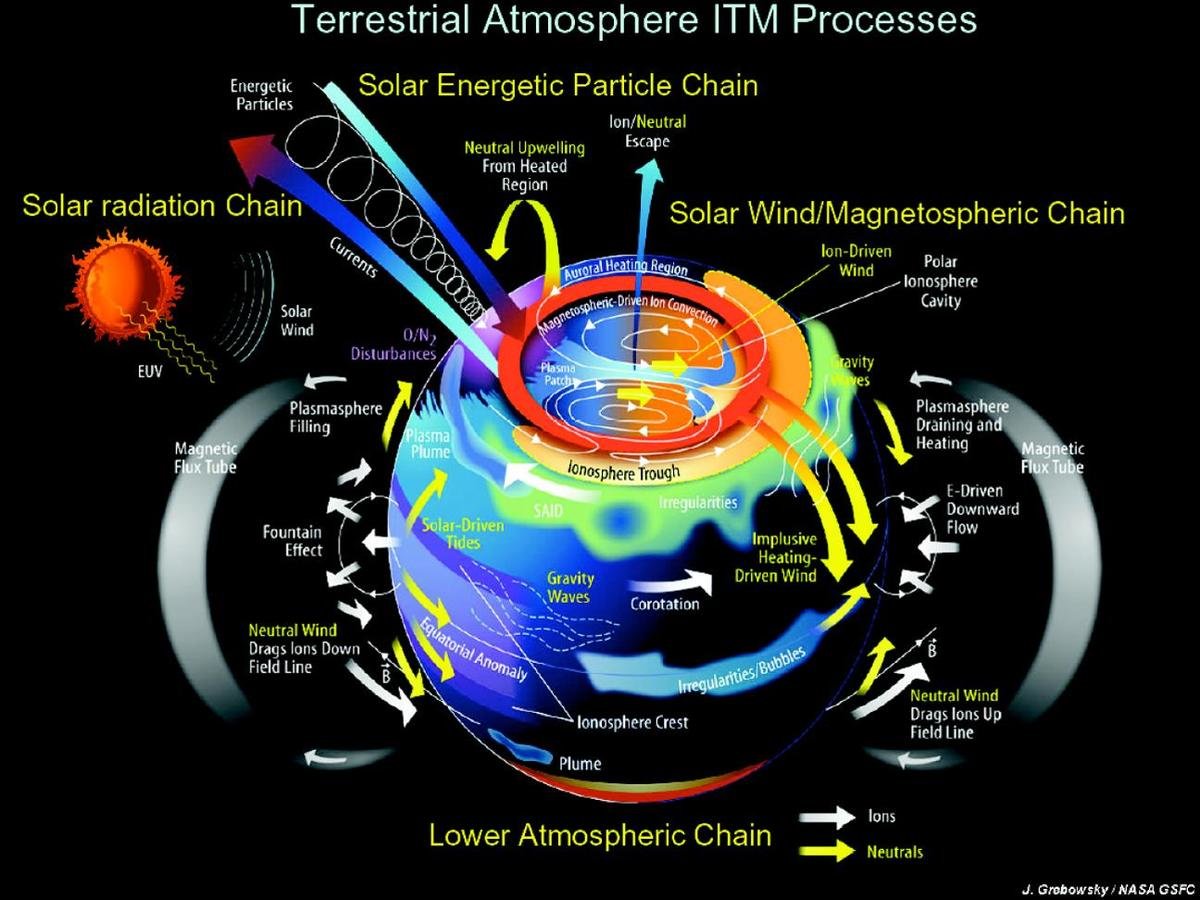
J. Grobowsky / NASA GSFC
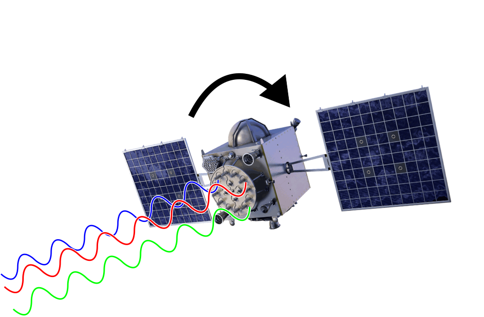
Ionosphere Effects on Electromagnetic Propagation
ionosphere = cold, collisionless, magnetized plasma
for L-band frequencies (1-2 GHz) refractive index given by:
n = 1 - \frac{1}{2} X \pm \mathcal{O}(\frac{1}{f^3})
\(f\) = wave frequency
\(N_e\) = plasma density
\(e\) = fundamental charge
\(m\) = electron rest mass
X = \frac{\omega_p^2}{\omega^2} \kern{1em}
\omega = 2 \pi f \kern{1em}
\omega_p = \sqrt{\frac{N_e e^2}{\epsilon_0 m}} \kern{1em}
radio source
ionosphere
phase shift / distortion

\(\epsilon_0\) = permittivity of free space
higher-order terms on the order of a few cm
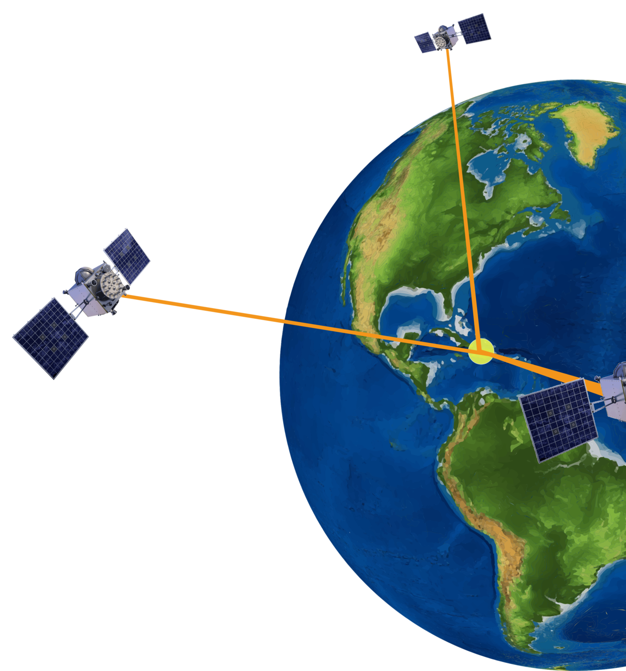
Global Navigation Satellite Systems (GNSS)
...a useful everyday radio source for geophysical remote-sensing!
GPS
GLONASS
Beidou
Galileio
...etc.
GPS - Global Positioning System
- 32-satellite constellation
- transmit dual-frequency BPSK-moduled signals
- new Block-IIF and next-gen Block-III satellites transmitting triple-frequency signals
| Signal | Frequency (GHz) |
|---|---|
| L1CA | 1.57542 |
| L2C | 1.2276 |
| L5 | 1.17645 |

GNSS Carrier Phase Observable
\Phi_i = r + c\Delta t + T + I_i + \lambda_i N_i + H_i + S_i + \epsilon_i
HARDWARE BIAS
IONOSPHERE RANGE ERROR
CARRIER AMBIGUITY
SYSTEMATIC ERRORS
FREQUENCY INDEPENDENT EFFECTS
STOCHASTIC ERRORS
accumulated phase (in meters) of demodulated GNSS signal at receiver for a particular satellite and signal carrier frequency \(f_i\)
Ionosphere Range Error
consider first-order term in ionosphere refractive index
I_i = \displaystyle \int_\text{rx}^\text{tx} \left(n - 1\right) \ ds
\approx -\frac{\kappa}{f_i^2} \displaystyle \int_\text{rx}^\text{tx} N_e \ ds
n \approx 1 - \frac{1}{2} X = 1-\frac{\kappa}{f_i^2} N_e
\kappa = \frac{e^2}{8\pi^2\epsilon_0 m_e} \approx 40.308
TOTAL ELECTRON CONTENT

rx
tx
plasma /
free electrons
units: \(\frac{\text{electrons}}{\text{m}^2}\)
often measured in TEC units:
1 \text{TECu} = 10^{16} \frac{\text{electrons}}{\text{m}^2}
Ionosphere Plasma Density
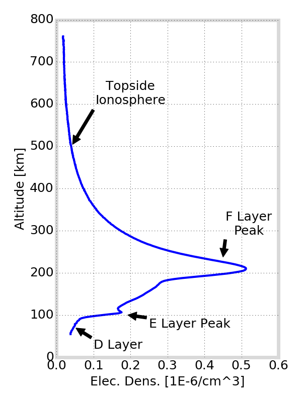
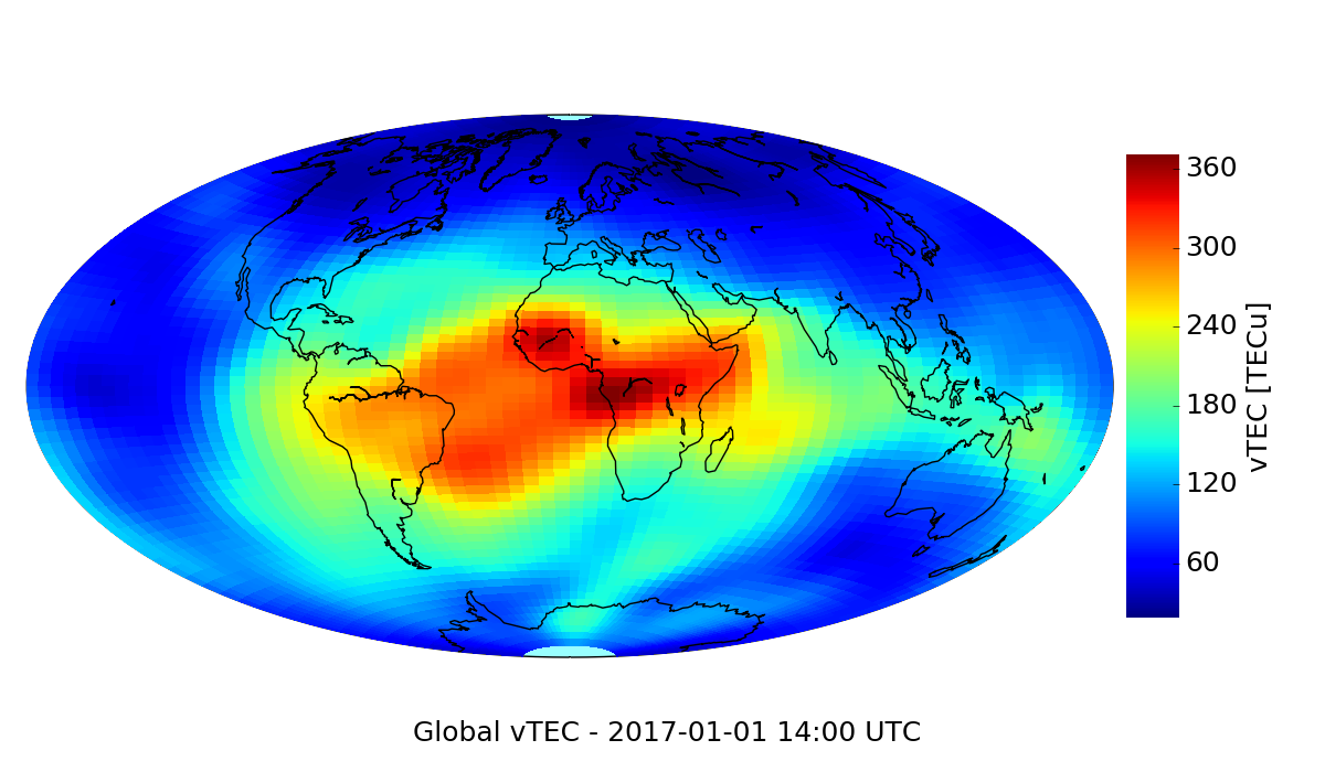
TEC and vertical TEC (vTEC) used to image plasma density structures
profile from CDAAC
image from Saito et al.
map from IGS
vertical distribution
horizontal distribution
travelling ionosphere disturbances (TIDs)
TEC
vTEC
TEC Estimation Using Dual-Frequency GNSS
\Phi_1 - \Phi_2 = \left(I_1 - I_2\right) + \left(\lambda_1 N_1 - \lambda_2 N_2\right) + \left(H_1 - H_2\right)
\approx -\kappa \left(\frac{1}{f_1^2} - \frac{1}{f_2^2}\right) \text{TEC} + \left(\lambda_1 N_1 - \lambda_2 N_2\right) + \Delta H_{1,2}
satellite and receiver inter-frequency hardware biases
neglecting systematic and stochastic error terms:
after resolving bias terms:
\text{TEC} = \displaystyle \frac{\Phi_2 - \Phi_1}{\kappa \left(\frac{1}{f_1^2} - \frac{1}{f_2^2}\right)}
carrier ambiguities
bias terms
Resolving Bias Terms
-
LAMBDA
-
code-carrier-levelling
-
[3] derives improved code-carrier leveling / ambiguity resolution using triple-frequency GNSS
carrier ambiguity resolution
hardware bias estimation
-
must apply ionosphere model
- e.g. global ionosphere model using data assimilation and receiver networks
- e.g. single receiver and linear 2D-gradient in vTEC (such as work by [2])
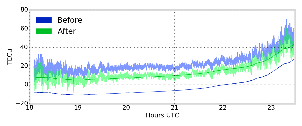
Example of L1/L2 TEC before and after code-carrier-levelling / ambiguity estimation, for satellite G01 and receiver at Poker Flat, Alaska.
2016-03-15
Examples of Dual-Frequency TEC Estimates

Poker Flat, Alaska, 2016-01-02
Using methods similar to [2] and [3] to solve for bias terms, we compute dual-frequency TEC estimate \(\text{TEC}_\text{L1,L2}\) and \(\text{TEC}_\text{L1,L5}\)
\(\text{TEC}_{\text{L1,L5}} - \text{TEC}_{\text{L1,L2}}\)
Poker Flat, Alaska, 2016-01-02

Can we characterize / find the source of these discrepancies?
Can we relate them to errors in dual-frequency TEC estimates?
Systematic Errors in GNSS Observations
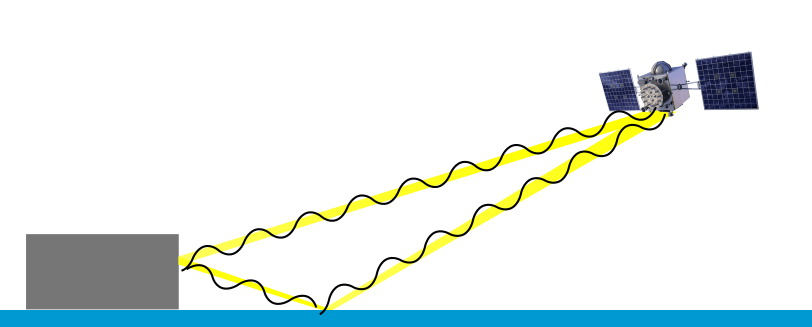
multipath
ray-path bending
higher-order ionosphere terms
antenna phase effects
hardware bias drifts
\(r \neq\) line-of-sight range
reflected signals interfere with primary signal at receiver \(\rightarrow\) causes fluctuations in phase / signal amplitude
\(H_i\) terms not constant
relative displacement of satellite antenna phase centers changes as satellite moves / rotates
need to consider orientation / strength of geomagnetic field
Objectives
Investigate the discrepancy in \(\text{TEC}_\text{L1,L5} - \text{TEC}_\text{L1,L2}\)
Derive optimal triple-frequency estimation of TEC
Provide a (partial) characterization of TEC estimate residual errors
Motivation
-
Push the boundaries of TID signature detection from earthquakes, explosions, etc.
-
Understand / address the errors in TEC estimates from low-elevation satellites
-
Improve user range error for precise positioning applications
Improve / understand TEC estimate precision
Approach
Apply framework to derive triple-frequency estimates of TEC and systematic errors
Develop framework for linear estimation of GNSS parameters
Relate to impact on TEC estimate error residuals
Background and Motivation
Linear Estimation of GNSS Parameters
TEC Estimate Error Residuals
Application to Real GPS Data
Simplified Carrier Phase Model
\Phi_i = G + I_i + S_i + \epsilon_i
zero-mean
normally-
distributed
zero-mean
neglect bias terms
By neglecting bias terms, we address estimation precision, rather than accuracy
\Phi_i = r + c\Delta t + T + I_i + \lambda_i N_i + H_i + S_i + \epsilon_i
"geometry" term
model parameters
\mathbf{\Phi} = \left[\Phi_1, \cdots, \Phi_m\right]^T
\mathbf{m} = \left[G, \text{TEC}, S_1, \cdots, S_m \right]^T
\mathbf{A} = \begin{bmatrix}
1 & -\frac{\kappa}{f_1^2} & 1 & 0 & \cdots & 0 \\
1 & -\frac{\kappa}{f_2^2} & 0 & 1 & \cdots & 0 \\
\vdots & & & & \ddots & \\
1 & -\frac{\kappa}{f_m^2} & 0 & \cdots & & 1
\end{bmatrix}
\mathbf{\epsilon} = [\epsilon_1, \cdots, \epsilon_m]^T
\mathbf{\Phi} = \mathbf{A} \mathbf{m} + \mathbf{\epsilon}
Linear Inverse Problem
observations
stochastic error
forward model
Linear Estimation
\mathbf{\hat{m}}
\mathbf{A^*} = \ ?
\mathbf{\hat{m}} \approx \mathbf{A^*} \mathbf{\Phi}
\mathbf{A}^T \left(\mathbf{A}\mathbf{A}^T\right)^{-1}
Poor results; treats each parameter with equal weight
We must apply a priori information about model parameters
model estimate
model estimator
A Priori Information
|G| \gg |I_i| \gg |S_i|
Under normal conditions, we know that:
G \sim
I \sim
S \sim
20,000 km
1 - 150 m
several cm
Using A Priori Information
We could apply \(|G| \gg |I_i| \gg |S_i|\) using Gaussian priors
Instead we derive each row separately:
\mathbf{A^*} =\begin{bmatrix}
\mathbf{C}_G \\
\mathbf{C}_\text{TEC} \\
\mathbf{C}_{S_1} \\
\vdots \\
\mathbf{C}_{S_m}
\end{bmatrix}
geometry estimator
TECu estimator
systematic-error estimators
estimator
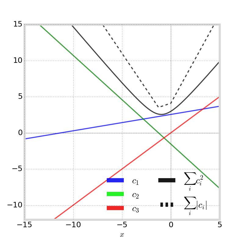
\mathbf{C} = \left[c_1, \cdots, c_m \right]^T \in \mathbb{R}^m
(written as row vectors here)
How to Choose Optimal \(\mathbf{C}\)
Goals:
1. produce desired parameter with unity coefficient
2. remove / reduce all other terms
Linear combination \(E\) given by inner-product:
E = \langle \mathbf{C} | \mathbf{\Phi} \rangle
Approach:
First, constrain \(\mathbf{C}\) to satisfy Goal 1
Then, constrain / optimize \(\mathbf{C}\) to achieve Goal 2
Linear Coefficient Constraints
Use one or two of the following constraints to reduce search space for optimal estimator coefficients:
\sum_i c_i = 0
\sum_i c_i = 1
geometry-free
geometry-estimator
\sum_i -\frac{\kappa}{f_i^2}c_i = 1
\sum_i \frac{c_i}{f_i^2} = 0
TEC-estimator
ionosphere-free
\Phi_i = G + I_i + S_i + \epsilon_i
Reduction of Error
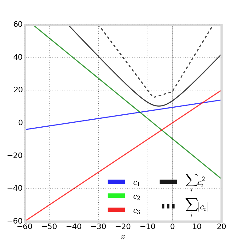
\mathbf{C}^* = \ \displaystyle \arg\min_\mathbf{C} \mathbf{C}^T \Sigma_\epsilon \mathbf{C}
Linear combination stochastic error variance:
\sigma_\epsilon^2 = \mathbf{C}^T \mathbf{\Sigma}_\epsilon \mathbf{C}
where \(\mathbf{\Sigma}_\epsilon\) is the covariance matrix between \(\mathbf{\epsilon}_i\)
Optimal \(\mathbf{C}\) for minimizing stochastic error variance:
\(\epsilon_i\) equal-amplitude and uncorrelated
\mathbf{C}^* = \ \displaystyle \arg\min_\mathbf{C} \sum_i c_i^2
TEC Estimator
1. apply TECu-estimator constraint
2. apply geometry-free constraint (since \(|G| \gg |I_i|\) )
Dual-Frequency Example
\Rightarrow c_1 = \displaystyle -\frac{1}{\kappa \left(\frac{1}{f_1^2} - \frac{1}{f_2^2}\right)}
\begin{aligned}
& -\frac{\kappa}{f_1^2}c_1 - \frac{\kappa}{f_2^2}c_2 = 1 \\[1em]
& c_1 + c_2 = 0 \Rightarrow c_1 = -c_2 \\[1em]
\Rightarrow & -\kappa c_1 \left(\frac{1}{f_1^2} - \frac{1}{f_2^2}\right) = 1
\end{aligned}
TEC-estimator
geometry-free
recall:
\text{TEC} = \displaystyle \frac{\Phi_2 - \Phi_1}{\kappa \left(\frac{1}{f_1^2} - \frac{1}{f_2^2}\right)}
Triple-Frequency TEC Estimator

Applying constraints yields following system of coefficients (with free parameter denoted \(x\):
\begin{aligned}
c_1 &= \frac{\frac{1}{\kappa} + x \left( \frac{1}{f_3^2} - \frac{1}{f_2^2}\right)}{\frac{1}{f_2^2} - \frac{1}{f_1^2}} \\[1em]
c_2 &= \frac{-\frac{1}{\kappa} - x \left( \frac{1}{f_3^2} - \frac{1}{f_1^2}\right)}{\frac{1}{f_2^2} - \frac{1}{f_1^2}}
\\[1em]
c_3 & = \ \ x
\end{aligned}
x^* = \frac{\frac{1}{\kappa}\left(\frac{2}{f_3^2} - \frac{1}{f_2^2} - \frac{1}{f_1^2}\right)}{\left(\frac{1}{f_1^2} - \frac{1}{f_2^2}\right)^2 + \left(\frac{1}{f_2^2} - \frac{1}{f_3^2}\right)^2 + \left(\frac{1}{f_3^2} - \frac{1}{f_1^2}\right)^2}
To satisfy \( \mathbf{C}^* = \ \displaystyle \arg\min_\mathbf{C} \sum_i c_i^2 \), choose
denote corresponding coefficient vector \(\mathbf{C}_{\text{TEC}_{1,2,3}}\) and its corresponding estimate \(\text{TEC}_{1,2,3}\)
TEC Estimator Using Triple-Frequency GPS

\begin{matrix}
\text{Estimate} & c_1 & c_2 & c_3 & \sum_i c_i^2 \\[.5em]
\text{TEC}_\text{L1,L2,L5} & 8.294 & -2.883 & -5.411 & 10.314 & \\
\text{TEC}_\text{L1,L5} & 7.762 & 0 & -7.762 & 10.977 & \\
\text{TEC}_\text{L1,L2} & 9.518 & -9.518 & 0 & 13.460 & \\
\text{TEC}_\text{L2,L5} & 0 & 42.080 & -42.080 & 59.510 &
\end{matrix}
\mathbf{C}_{\text{TEC}_\text{L1,L2,L5}}
\mathbf{C}_{\text{TEC}_\text{L1,L5}}
\mathbf{C}_{\text{TEC}_\text{L1,L2}}
\mathbf{C}_{\text{TEC}_\text{L2,L5}}
Geometry Estimator
\begin{matrix}
c_1 = & \frac{-\frac{1}{f_2^2} + x \left(\frac{1}{f_2^2} - \frac{1}{f_3^2}\right)}{\frac{1}{f_1^2} - \frac{1}{f_2^2}} \\
c_2 = & \frac{\frac{1}{f_1^2} - x \left(\frac{1}{f_1^2} - \frac{1}{f_3^2}\right)}{\frac{1}{f_1^2} - \frac{1}{f_2^2}} \\
c_3 = & x
\end{matrix}
For triple-frequency GNSS:
1. apply geometry-estimator constraint
2. apply ionosphere-free constraint since \(I_i\) are the next-largest terms
x^* = \frac{\frac{1}{\kappa}\left(\frac{2}{f_3^2} - \frac{1}{f_2^2} - \frac{1}{f_1^2}\right)}{\left(\frac{1}{f_1^2} - \frac{1}{f_2^2}\right)^2 + \left(\frac{1}{f_2^2} - \frac{1}{f_3^2}\right)^2 + \left(\frac{1}{f_3^2} - \frac{1}{f_1^2}\right)^2}
To satisfy \( \mathbf{C}^* = \ \displaystyle \arg\min_\mathbf{C} \sum_i c_i^2 \),
We call this coefficient vector \(\mathbf{C}_{G_{1,2,3}}\) and its corresponding estimate \(G_{1,2,3}\)
the optimal "ionosphere-free combination"
Geometry Estimator Using Triple-Frequency GPS
\begin{matrix}
\text{Estimate} & c_1 & c_2 & c_3 & \sum_i c_i^2 \\[.5em]
G_\text{L1,L2,L5} & 2.327 & -0.360 & -0.967 & 2.546 \\
G_\text{L1,L5} & 2.261 & 0 & -1.261 & 2.588 \\
G_\text{L1,L2} & 2.546 & -1.546 & 0 & 2.978 \\
G_\text{L2,L5} & 0 & 12.255 & -11.255 & 16.639
\end{matrix}

\mathbf{C}_{G_\text{L1,L2,L5}}
\mathbf{C}_{G_\text{L1,L5}}
\mathbf{C}_{G_\text{L1,L2}}
\mathbf{C}_{G_\text{L2,L5}}
Systematic Error Estimator
Since \(|G| \gg |I_i| \gg |S_i|\), must apply both geometry-free and ionosphere-free constraints
For triple-frequency GNSS:
\begin{aligned}
c_1 & = \ \ x \frac{\frac{1}{f_3^2} - \frac{1}{f_2^2}}{\frac{1}{f_2^2} - \frac{1}{f_1^2}} \\[1em]
c_2 & = - x \frac{\frac{1}{f_3^2} - \frac{1}{f_1^2}}{\frac{1}{f_2^2} - \frac{1}{f_1^2}} \\[1em]
c_3 & = \ \ x
\end{aligned}
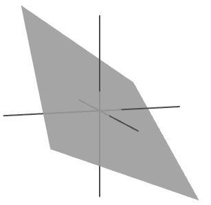
system is linear subspace
note this requires \(m \ge 3\)

Geometry-Ionosphere-Free Combination
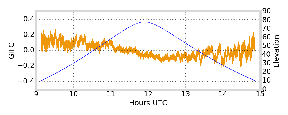
We call the linear combination that applies both geometry-free and ionosphere-free constraints the geometry-ionosphere-free combination (GIFC)
FACT: The difference between any two TEC estimates produces some scaling of the GIFC
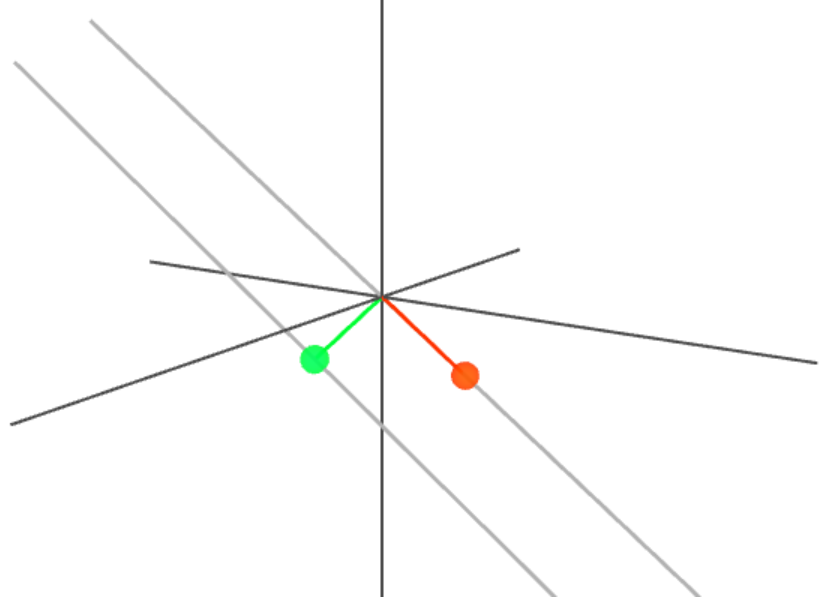
FACT: \(\mathbf{C}_\text{GIFC}\) and \(\mathbf{C}_{\text{TEC}_{1,2,3}}\) are perpendicular, i.e.
\langle \mathbf{C}_\text{GIFC} | \mathbf{C}_{\text{TEC}_{1,2,3}} \rangle = 0
FACT:
\frac{\langle \mathbf{C}_\text{TEC} | \mathbf{C}_{\text{TEC}_{1,2,3}} \rangle}{|| \mathbf{C}_{\text{TEC}_{1,2,3}} ||} = || \mathbf{C}_{\text{TEC}_{1,2,3}} ||
i.e. \(\mathbf{C}_\text{TEC} \) projected onto direction \(\mathbf{C}_{\text{TEC}_{1,2,3}}\) lands at \(\mathbf{C}_{\text{TEC}_{1,2,3}} \)
\mathbf{C}_{\text{TEC}_{1,2,3}}
\mathbf{C}_\text{GIFC}
GIFC Triple-Frequency GPS
\begin{aligned}
\mathbf{C}_{\text{GIFC}_\text{L1,L2,L5}} & = \mathbf{C}_{\text{TEC}_{\text{L1,L5}}} - \mathbf{C}_{\text{TEC}_{\text{L1,L2}}} \\[1em]
& = \left[-1.756, 9.520, -7.764\right]^T
\end{aligned}
We (arbitrarily) choose:
Note: the triple-frequency GIFC does not have a well-defined unit.
GIFC in our results section have the scaling shown here.
Background and Motivation
Linear Estimation of GNSS Parameters
TEC Estimate Error Residuals
Application to Real GPS Data
Estimate Residual Error
Define the error residual vector \(\mathbf{R}\) with components:
The residual error impacting the TEC estimate is:
R_{\text{TEC}} = \langle \mathbf{C}_{\text{TEC}} | \mathbf{R} \rangle
\text{GIFC} = \langle \mathbf{C}_{\text{GIFC}} | \mathbf{R} \rangle
Note that:
R_i = S_i + \epsilon_i
A Convenient Basis
We transform \(\mathbf{R}\) using the orthonormal basis:
\mathbf{U}_1 = \frac{\mathbf{C}_{\text{TEC}_{1,2,3}}}{||\mathbf{C}_{\text{TEC}_{1,2,3}}||}
\mathbf{U}_2 = \frac{\mathbf{C}_\text{GIFC}}{||\mathbf{C}_\text{GIFC}||}
\mathbf{U}_3 = \mathbf{U}_1 \times \mathbf{U}_2
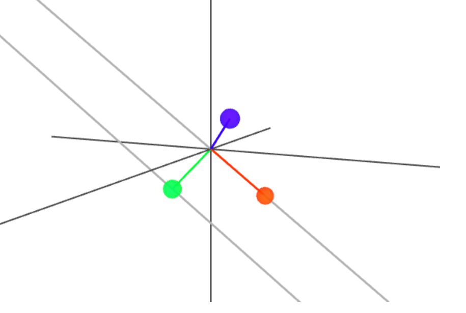
\mathbf{U} = \begin{bmatrix} \mathbf{U}_1 \\ \mathbf{U}_2 \\ \mathbf{U}_3 \end{bmatrix}
\mathbf{R}' = \mathbf{U} \mathbf{R}
Note that \(\mathbf{U}_3 \perp \mathbf{C}_\text{TEC} \) since \(\mathbf{U}_1\) and \(\mathbf{U}_2\) span the geometry-free plane
R_i' = \langle \mathbf{U}_i | \mathbf{R} \rangle
R_1' = \frac{R_{\text{TEC}_{1,2,3}}}{||\mathbf{C}_{\text{TEC}_{1,2,3}}||}
R_2' = \frac{\text{GIFC}}{||\mathbf{C}_\text{GIFC}||}
Note that:
TEC Estimate Residual Error
common TEC estimate residual error component
GIFC residual error component
\begin{aligned}
R_\text{TEC} & = \langle \mathbf{U} \mathbf{C}_\text{TEC} | \mathbf{U} \mathbf{R} \rangle \\[1em]
& = \langle \mathbf{U}_1 | \mathbf{C}_\text{TEC} \rangle R_1' + \langle \mathbf{U}_2 | \mathbf{C}_\text{TEC} \rangle R_2' \\[1em]
& = R_{\text{TEC}_{1,2,3}} + \frac{\langle \mathbf{C}_\text{GIFC} | \mathbf{C}_\text{TEC} \rangle}{||\mathbf{C}_\text{GIFC}||^2} R_\text{GIFC}
\end{aligned}
Express \(R_\text{TEC}\) as residual error components in transformed coordinate system:
\mathbf{U}_1 = \frac{\mathbf{C}_{\text{TEC}_{1,2,3}}}{||\mathbf{C}_{\text{TEC}_{1,2,3}}||}
\mathbf{U}_2 = \frac{\mathbf{C}_\text{GIFC}}{||\mathbf{C}_\text{GIFC}||}
\langle \mathbf{U}_3 | \mathbf{C}_\text{TEC} \rangle = 0
TEC Estimate Residual Error Discussion
Term \( \frac{\langle \mathbf{C}_\text{GIFC} | \mathbf{C}_\text{TEC} \rangle}{||\mathbf{C}_\text{GIFC}||^2} \) = amplitude of GIFC residual error component in TEC estimate
Term \(R_{\text{TEC}_{1,2,3}}\) = unobservable "TEC-like" residual error component
\(\text{TEC}_{1,2,3}\) is optimal in the sense that it completely removes the GIFC component of residual error
But can we say anything about the overall TEC estimate residual error?
Argument for Using GIFC to Assess Overall Residual Error
Assume \(\mathbf{R}\) has an overall distribution that is joint symmetric about the origin with distribution function \(f_R(x)\)
The distribution of a scaled version \(a \mathbf{R}\) for some scalar \(a\) is \(f_R (\frac{x}{a})\)
By definition, \(\mathbf{U}\mathbf{R} \sim \) symmetric with \(f_R(x) \) for any orthonormal transformation \(\mathbf{U}\)
\(R_i\) equal amplitude and uncorrelated
f_{R_\text{TEC}}(x) = f_{R}\left( \frac{x}{||\mathbf{C}_\text{TEC} ||} \right)
f_\text{GIFC}(x) = f_{R}\left( \frac{x}{||\mathbf{C}_\text{GIFC} ||} \right)
f_{R_\text{TEC}} (x) = f_\text{GIFC}\left( \frac{||\mathbf{C}_\text{GIFC}||}{||\mathbf{C}_\text{TEC} ||} x \right)
Overall TEC Residual Error Discussion
The assumption that \(\mathbf{R}\) has joint symmetric distribution is wrong
We can do better by carefully assessing a priori knowledge about the error components in each \(\Phi_i\)
- investigating GIFC is first-step in this process
\(f_{R_\text{TEC}}(x) = f_\text{GIFC} \left(\frac{||\mathbf{C}_\text{GIFC}||}{||\mathbf{C}_\text{TEC}||} x \right) \) is a coarse approximation
- relates deviations as: \(\text{dev} R_\text{TEC} \approx \frac{||\mathbf{C}_\text{TEC}||}{||\mathbf{C}_\text{GIFC}||} \text{dev} \ \text{GIFC} \)
- could be very wrong if \(R_{\text{TEC}_{1,2,3}} \gg GIFC \)
Relation Between GIFC and TEC Estimate Residual Errors
\begin{matrix}
\text{Estimate} & \frac{\langle \mathbf{C}_\text{GIFC} | \mathbf{C}_\text{TEC} \rangle}{||\mathbf{C}_\text{GIFC}||^2} & \frac{||\mathbf{C}_\text{TEC}||}{||\mathbf{C}_\text{GIFC}||} \\
\text{TEC}_\text{L1,L2,L5} & 0 & 0.831 \\
\text{TEC}_\text{L1,L5} & 0.303 & 0.885 \\
\text{TEC}_\text{L1,L2} & -0.697 & 1.085 \\
\text{TEC}_\text{L2,L5} & 4.723 & 4.796
\end{matrix}
amplitude of GIFC error signal in TEC residual
relates deviation in GIFC and TEC residual
Background and Motivation
Linear Estimation of GNSS Parameters
TEC Estimate Error Residuals
Application to Real GPS Data
Experiment Data
GPS Lab high-rate GNSS data collection network
- Alaska, Hong Kong, Peru
- 2013, 2014, 2015, 2016
- Septentrio PolarXs
- 1 Hz GPS L1/L2/L5 measurements

Data Alignment and Correction
GPS orbital period \(\approx\) 1/2 sidereal day
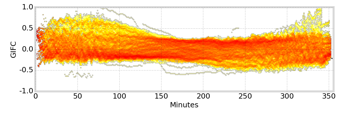
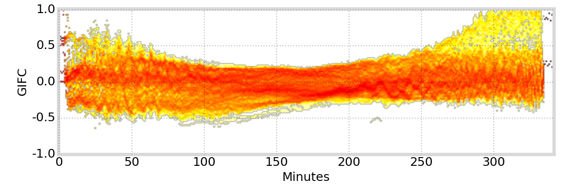
Outlier segments (\(|\text{GIFC}| > 2\)) are removed from analysis
align data by sidereal day = 23h 55m 54.2 s
must remove jumps in GIFC data due to ionosphere activity / multipath / interference
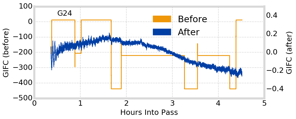
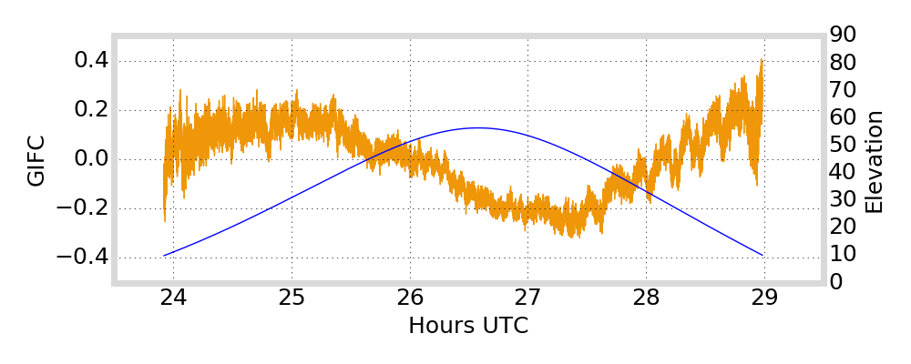
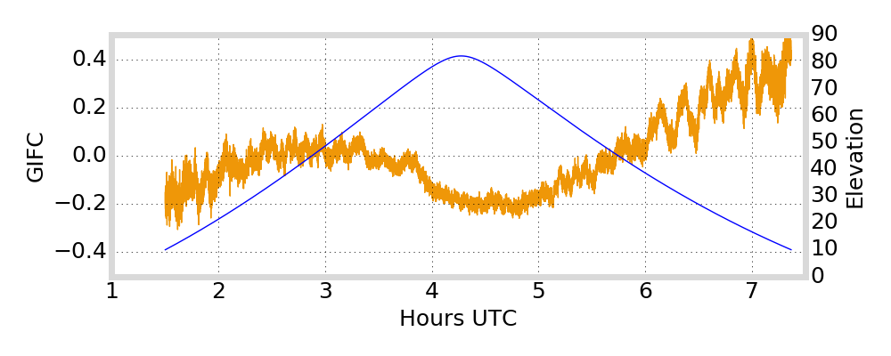
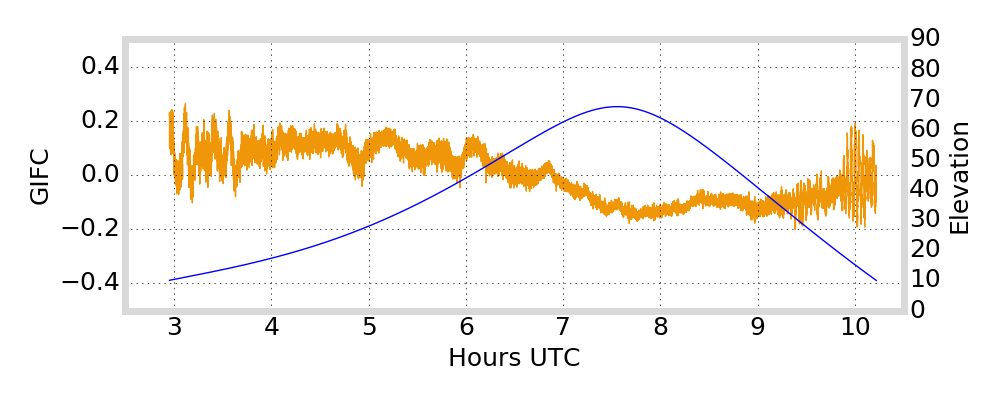
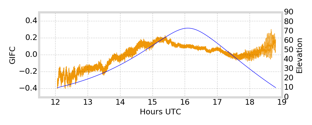
GIFC Examples
Alaska
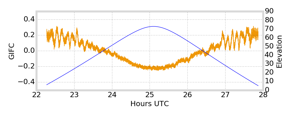
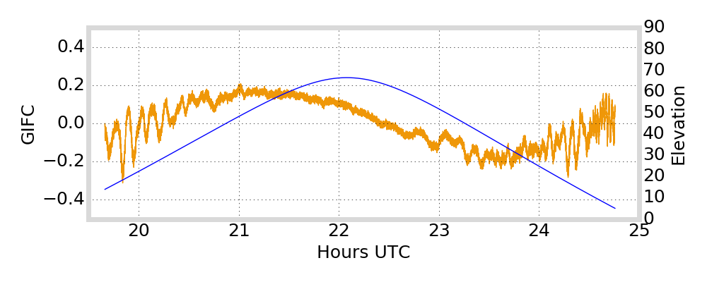

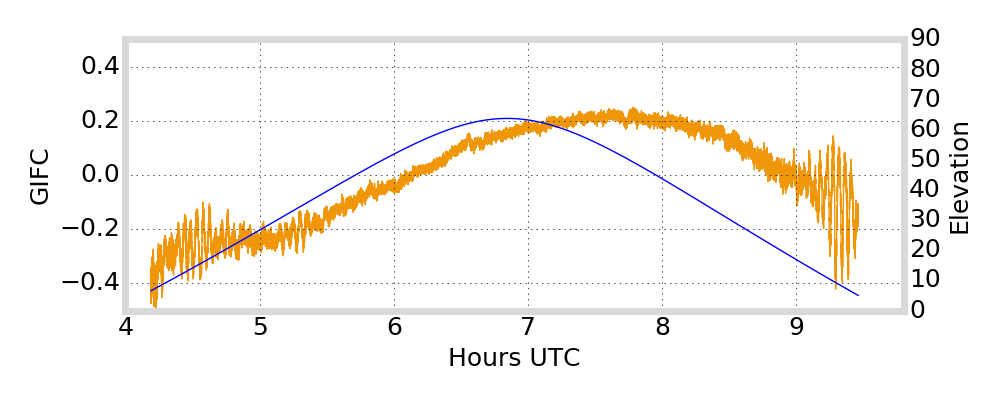
G01
G24
G25
G27
GIFC Examples
Hong Kong

G01
G24
G25
G27
GIFC Examples
Peru


G01
G24
G25
G27

GIFC Calendar
Alaska


G01
G24
G25
G27
GIFC Calendar
Hong Kong

G01
G24
G25
G27
GIFC Calendar
Peru
G01
G24
G25
G27
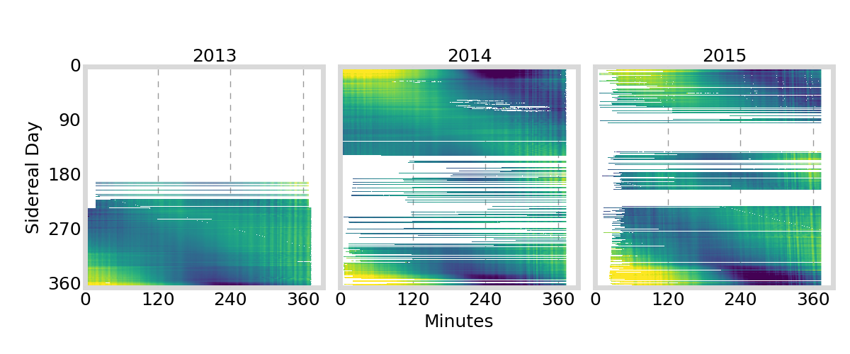
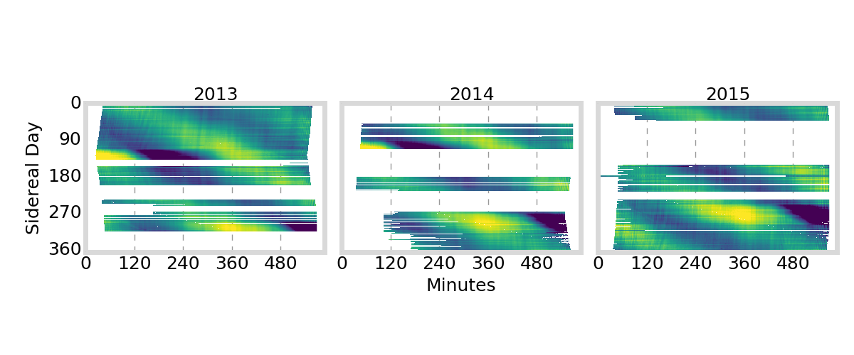
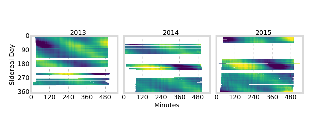
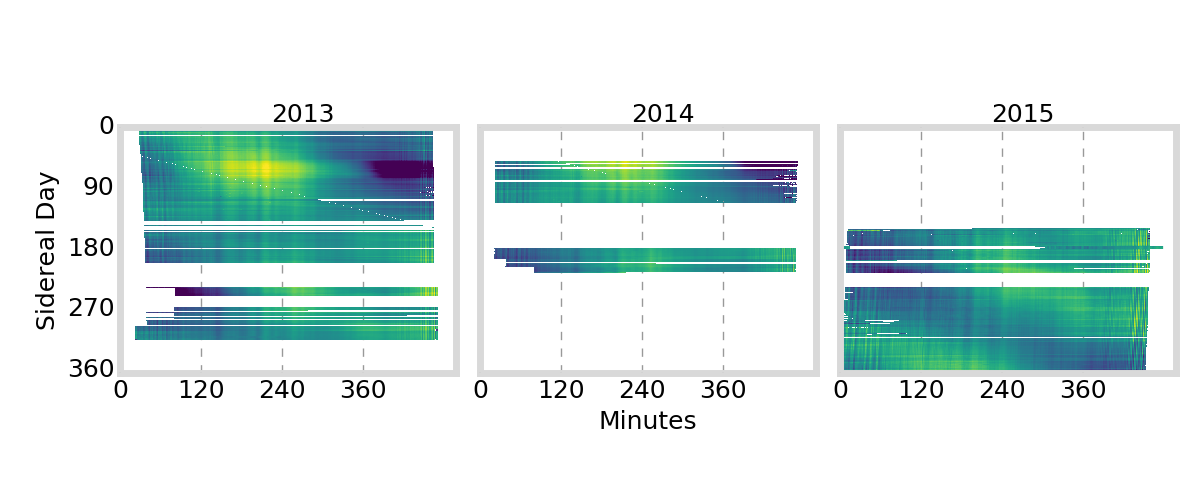
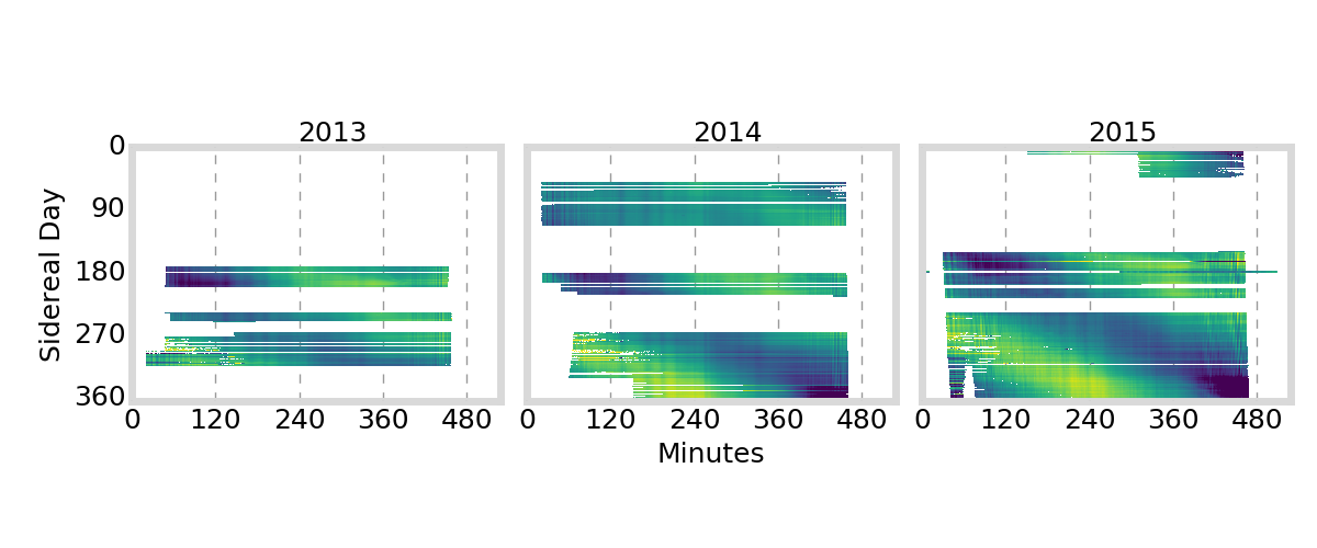
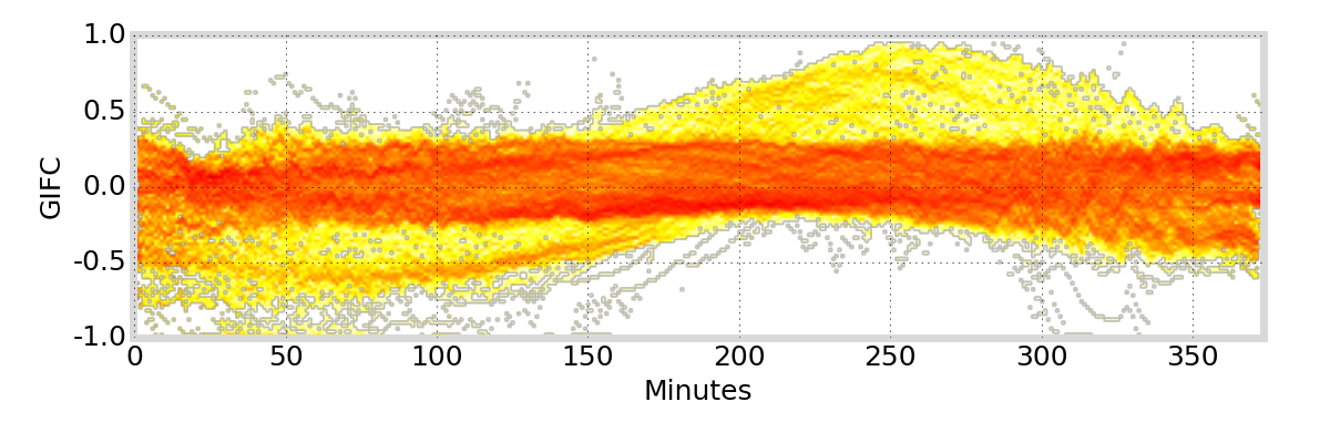
Satellite Antenna Phase Effects?
antenna phase effects
relative displacement of satellite antenna phase centers changes as satellite moves / rotates


angle cosine between Earth center, satellite, and Sun
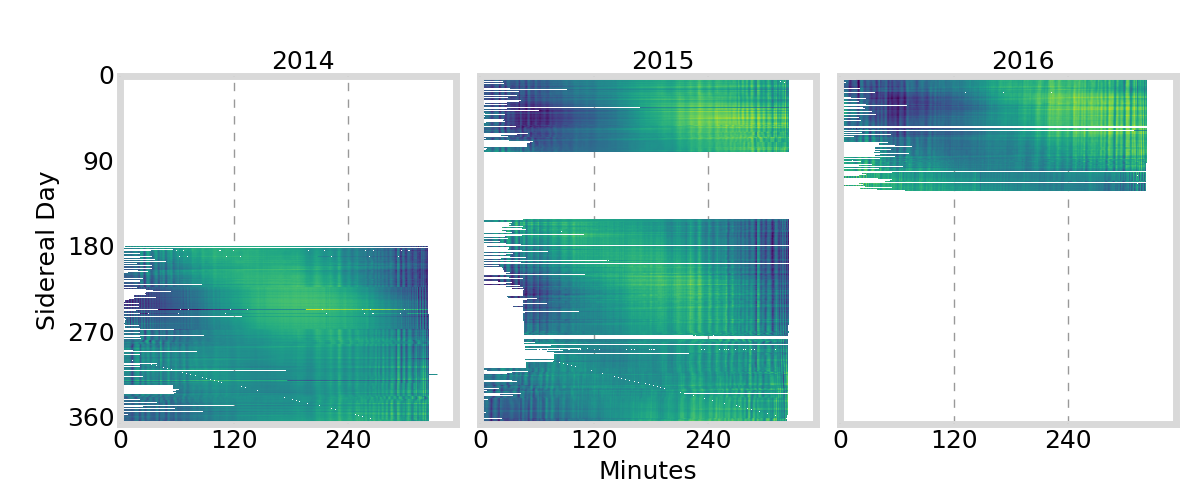
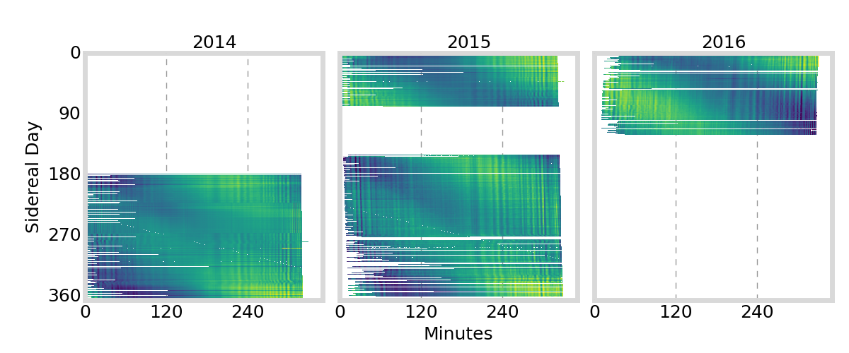
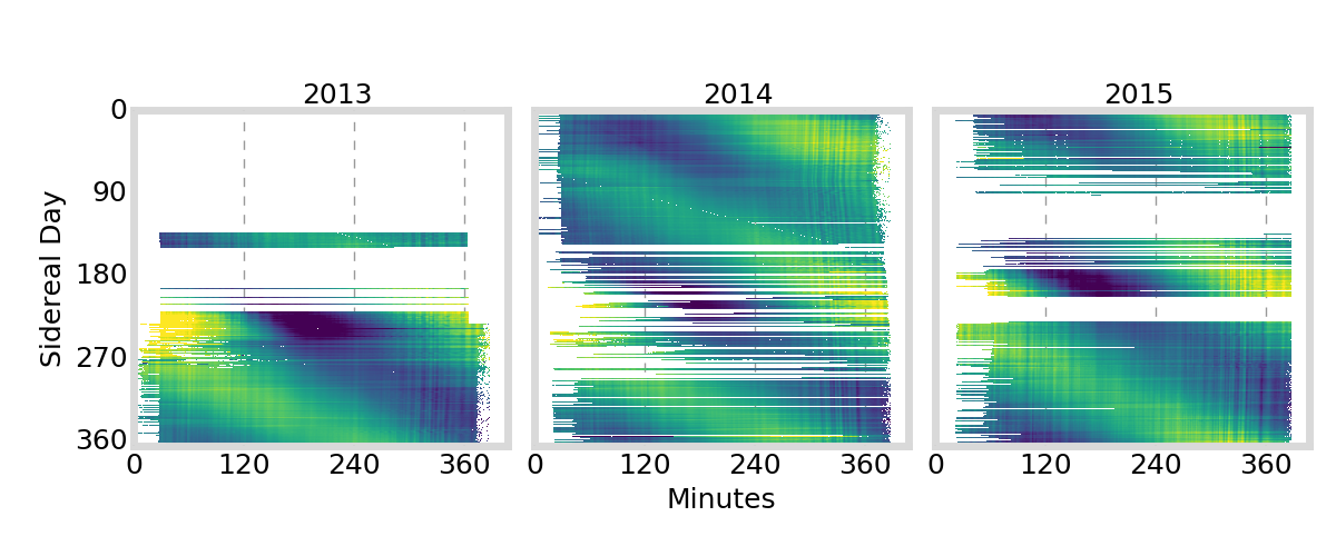
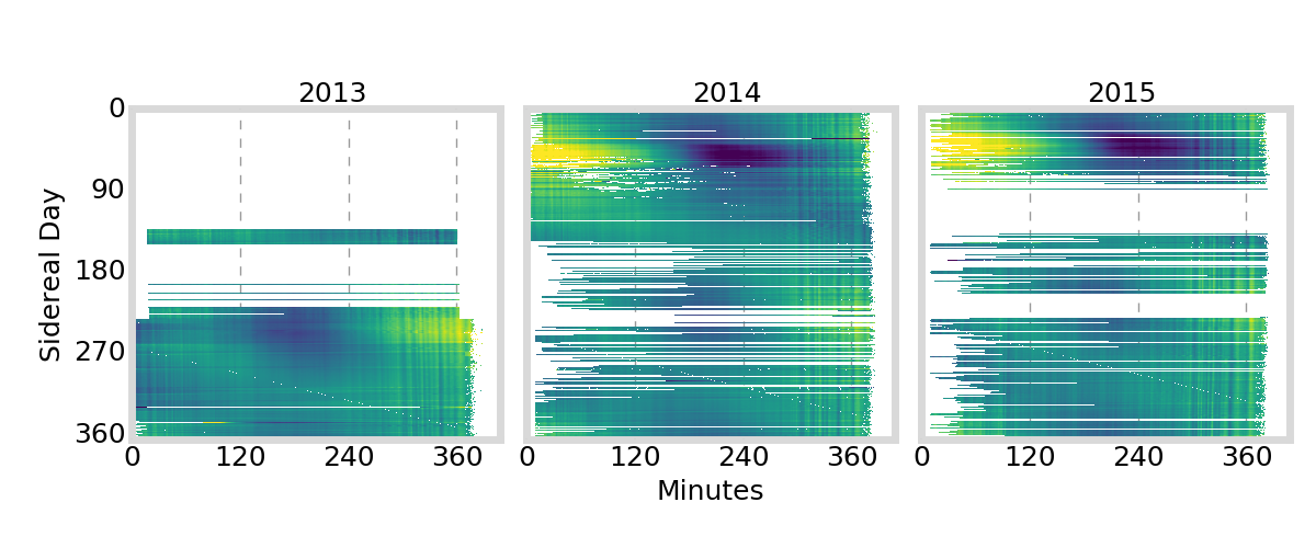
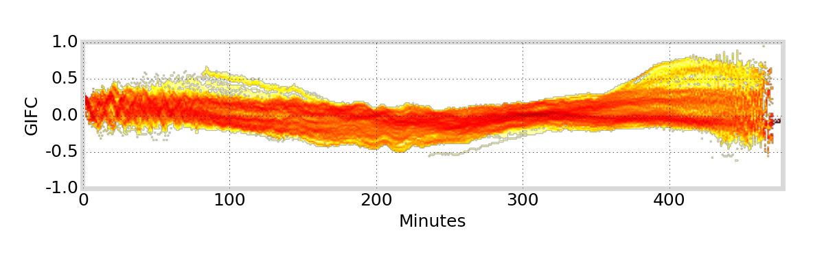
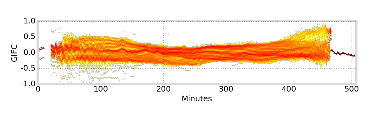
GIFC Heatmap
Alaska
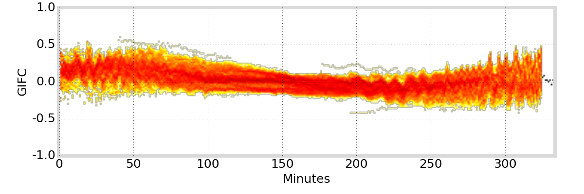
G01
G24
G25
G27
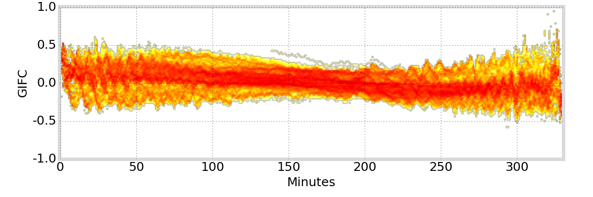
GIFC Heatmap
Hong Kong
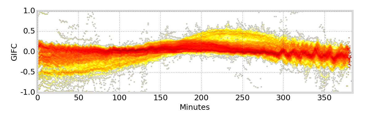
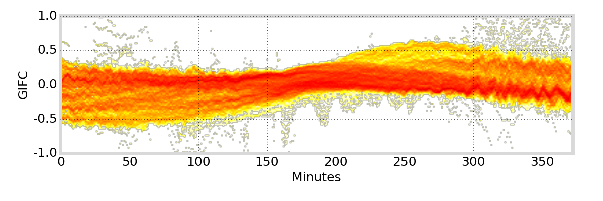
G01
G24
G25
G27
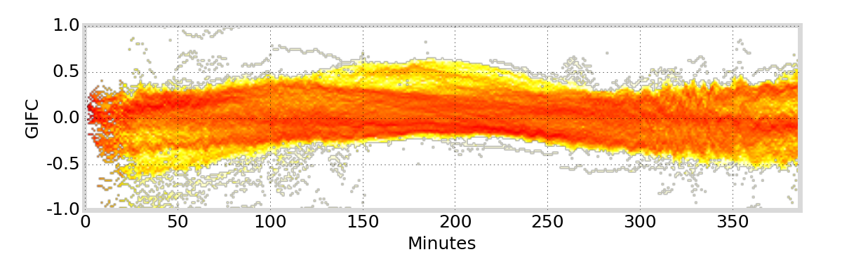
GIFC Heatmap
Peru
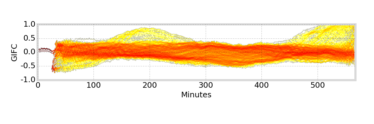
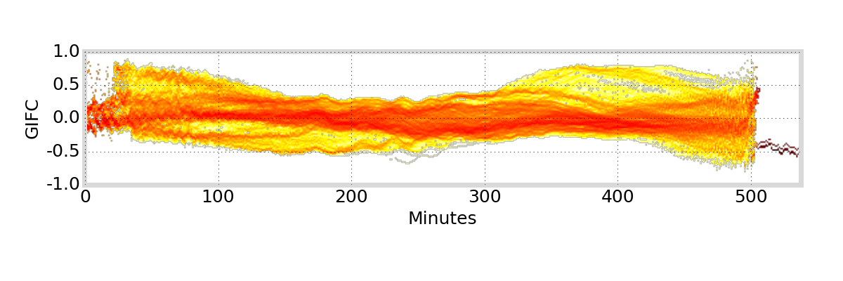
G01
G24
G25
G27
GIFC Deviations and TEC Residual Error Estimates
\begin{matrix}
\text{Percentile} & \text{Overall} \\
50 & 0.11 \\
75 & 0.19 \\
90 & 0.21 \\
\end{matrix}
\begin{matrix}
\text{Percentile} & \kern{5em} & \text{TEC}_\text{L1,L5} & \text{TEC}_\text{L1,L2} & \text{TEC}_\text{L2,L5} \\
50 & & 0.033 & 0.077 & 0.520 \\
75 & & 0.058 & 0.132 & 0.897 \\
90 & & 0.064 & 0.146 & 0.992
\end{matrix}
\begin{matrix}
\text{Percentile} & \text{TEC}_\text{L1,L2,L5} & \text{TEC}_\text{L1,L5} & \text{TEC}_\text{L1,L2} & \text{TEC}_\text{L2,L5} \\
50 & 0.091 & 0.097 & 0.119 & 0.528 \\
75 & 0.158 & 0.168 & 0.206 & 0.911 \\
90 & 0.175 & 0.186 & 0.228 & 1.007
\end{matrix}
\frac{\langle \mathbf{C}_\text{GIFC} | \mathbf{C}_\text{TEC} \rangle}{||\mathbf{C}_\text{GIFC}||^2}
\frac{||\mathbf{C}_\text{TEC}||}{||\mathbf{C}_\text{GIFC}||}
GIFC deviation multiplied by scaling factor
[TECu]
GIFC percentile deviations computed over aggregate of all data
Recap
simple phase observation model (ignore biases)
methodology for choosing optimal linear estimators
triple-frequency
\(\text{TEC}_{1,2,3}\)
GIFC
optimal?
characterize / relate to \(R_\text{TEC}\)
Discussion
\(\text{TEC}_\text{L1,L2}\) residual error on order of 0.2 TECu
- includes large-scale trend \(\rightarrow\) for TID detection, trend is removed and precision improves
- [4] cites 0.05 TECu fluctuations to be above noise for TID detection
Improvement of \(\text{TEC}_\text{L1,L2,L5}\) over \(\text{TEC}_\text{L1,L5}\) seems minor:
||\mathbf{C}_{\text{TEC}_\text{L1,L2,L5}}|| = 10.314
||\mathbf{C}_{\text{TEC}_\text{L1,L5}}|| = 10.977
||\mathbf{C}_{\text{TEC}_\text{L1,L2}}|| = 13.460
...but it does eliminate GIFC component in TEC residual error
Next Steps
Use characterization of GIFC to address residual errors
Can we obtain and apply better information on residual error components \(R_i\)?
Is the GIFC trend variation due to satellite antenna phase effects?
Can we use GIFC to validate mitigation techniques for multipath, higher-order ionosphere terms, ray-path bending, antenna phase effects?
\(\rightarrow\) enable TEC estimation from low-elevation satellites
Acknowledgements
This research was supported by the Air Force Research Laboratory and NASA.
Thank you to my advisor, committee members, and all who provided me with feedback and criticism!
References
[1] Saito A., S. Fukao, and S. Miyazaki, High resolution mapping of TEC perturbations with the GSI GPS network over Japan, Geophys. Res. Lett., 25, 3079-3082, 1998.
[2] Bourne, Harrison W. An algorithm for accurate ionospheric total electron content and receiver bias estimation using GPS measurements. Diss. Colorado State University. Libraries, 2016.
[3] Spits, Justine. Total Electron Content reconstruction using triple frequency GNSS signals. Diss. Université de Liège, Belgique, 2012.
[4] M. Nishioka, A. Saito, and T. Tsugawa, “Occurrence characteristics of plasma bubble derived from global ground-based GPS receiver networks,” Journal of Geophysical
Research: Space Physics, vol. 113, no. A5, 2008.
Optimal Linear Combinations of GNSS Phase Observables to Improve and Assess TEC Estimation Precision
By Brian Breitsch


