The non-Gaussian mapping from redshift to real space

In collaboration with:
Baojiu Li, Carlton Baugh, Alexander Eggemeier, Pauline Zarrouk, Takahiro Nishimichi and Masahiro Takada
Carolina Cuesta-Lazaro

Space-time
geometetry
Energy content
Adding new degrees of freedom
- To the energy content (dynamic) DARK ENERGY
- To the way space-time geometry reacts to the energy content MODIFIED GRAVITY (FIFTH FORCES)
?
Fifth forces modify structure growth
GROWTH
- GRAVITY
- FIFTH FORCE
+ EXPANSION
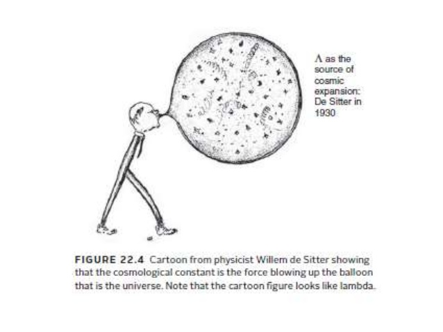
Credit: Cartoon depicting Willem de Sitter as Lambda from Algemeen Handelsblad (1930).
GR vs MG
PECULIAR VELOCITIES
GALAXY SURVEYS
(\vec{\theta}_i, z_i)
z_i = z_{\mathrm{Cosmological} }
+ z_{\mathrm{Doppler}}
\chi(z) = \int_0^z \frac{dz'}{H(z')}
+ \frac{v_{\mathrm{pec}}}{aH(a)}

\chi_i
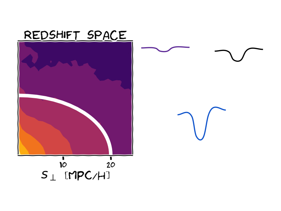
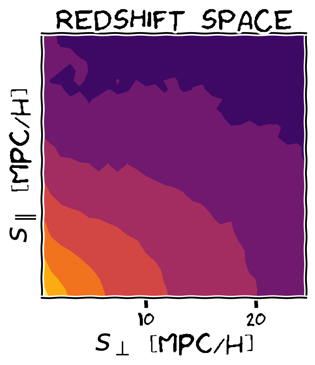
Streaming Model of Redshift Space Distortions
1+\xi(s_\perp, s_\parallel) = \int dr_\parallel \left(1 + \xi(r)\right) \mathcal{P}(v_\parallel=s_\parallel-r_\parallel|r_\perp, r_\parallel)
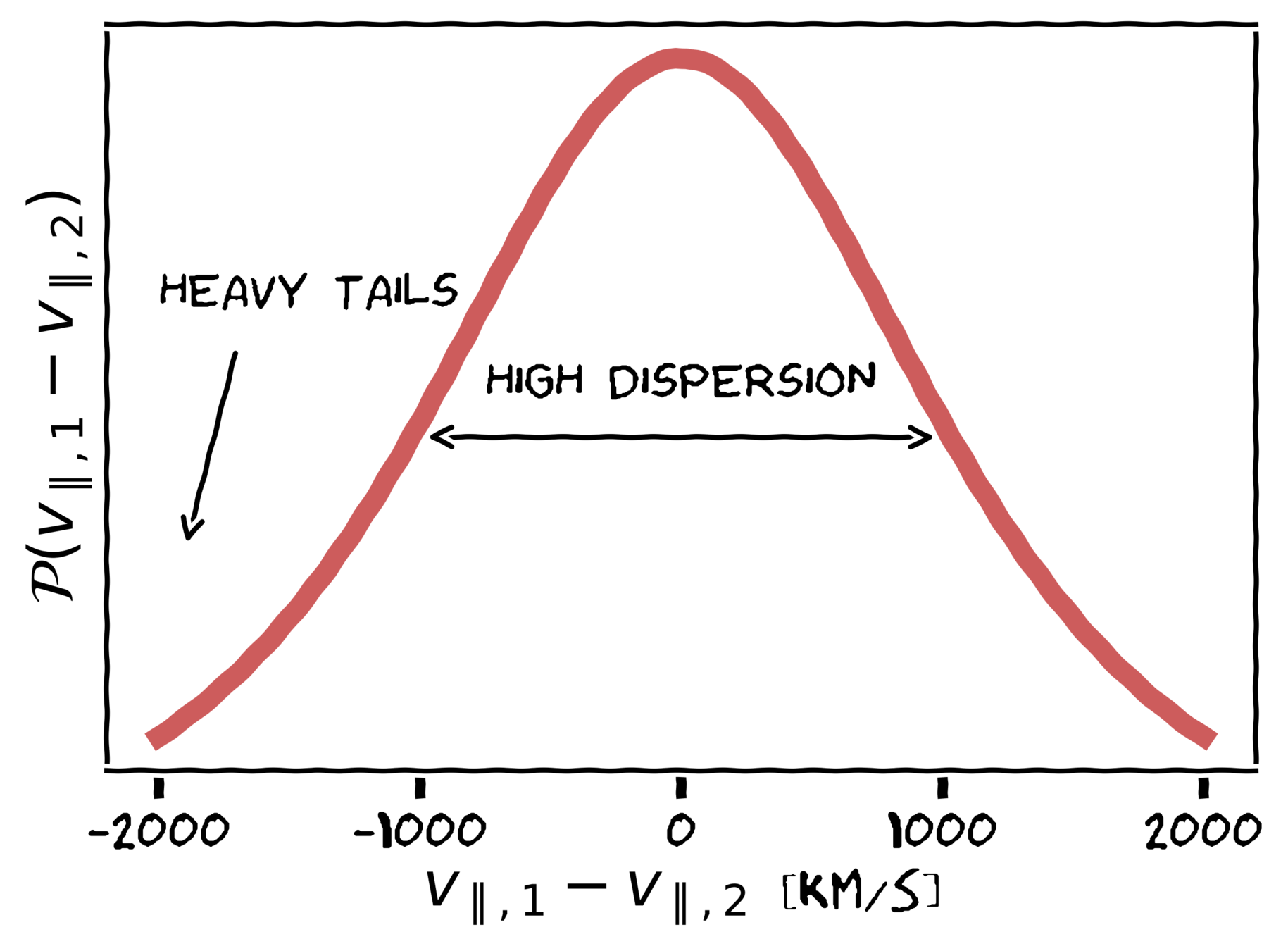
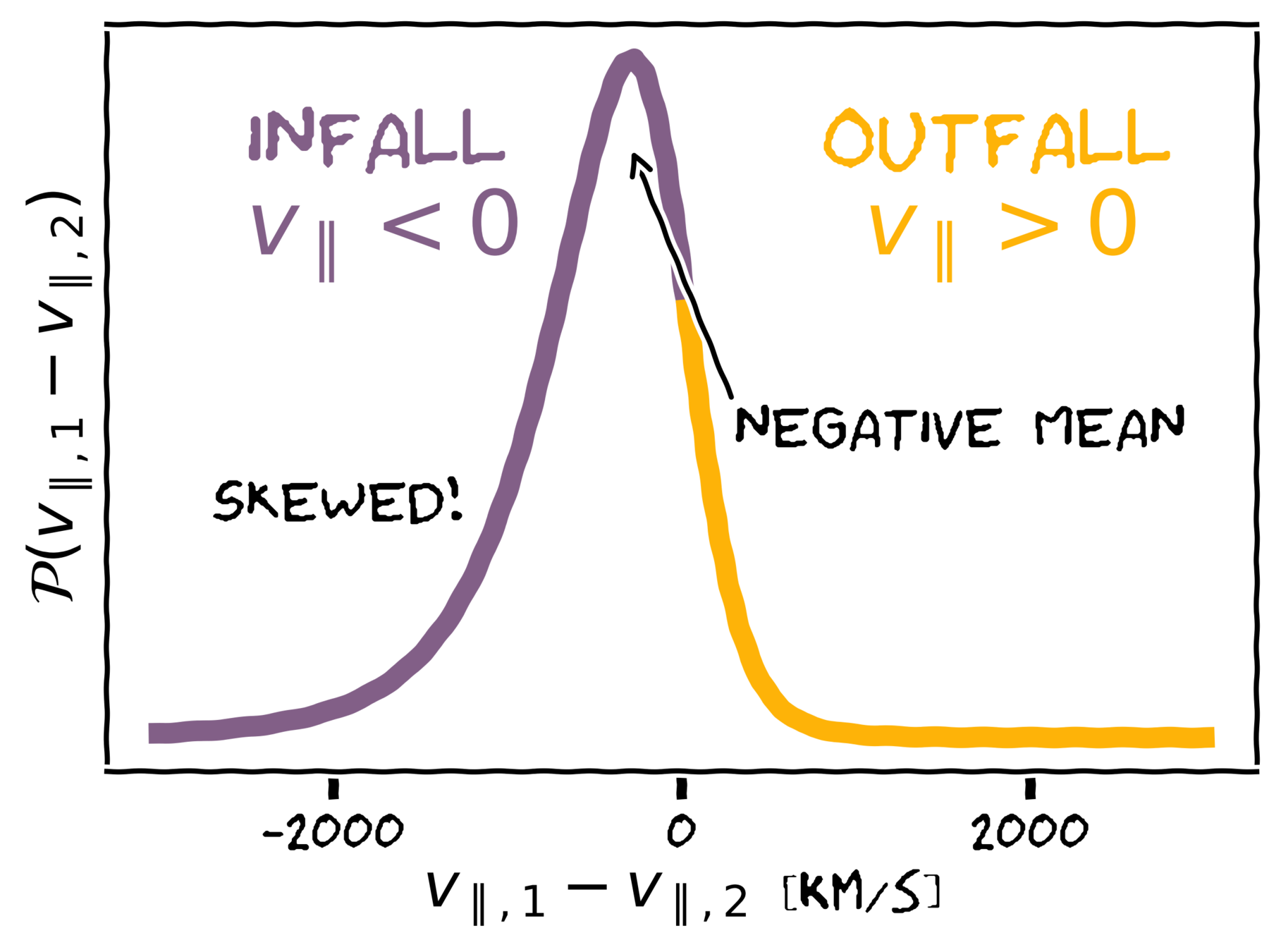
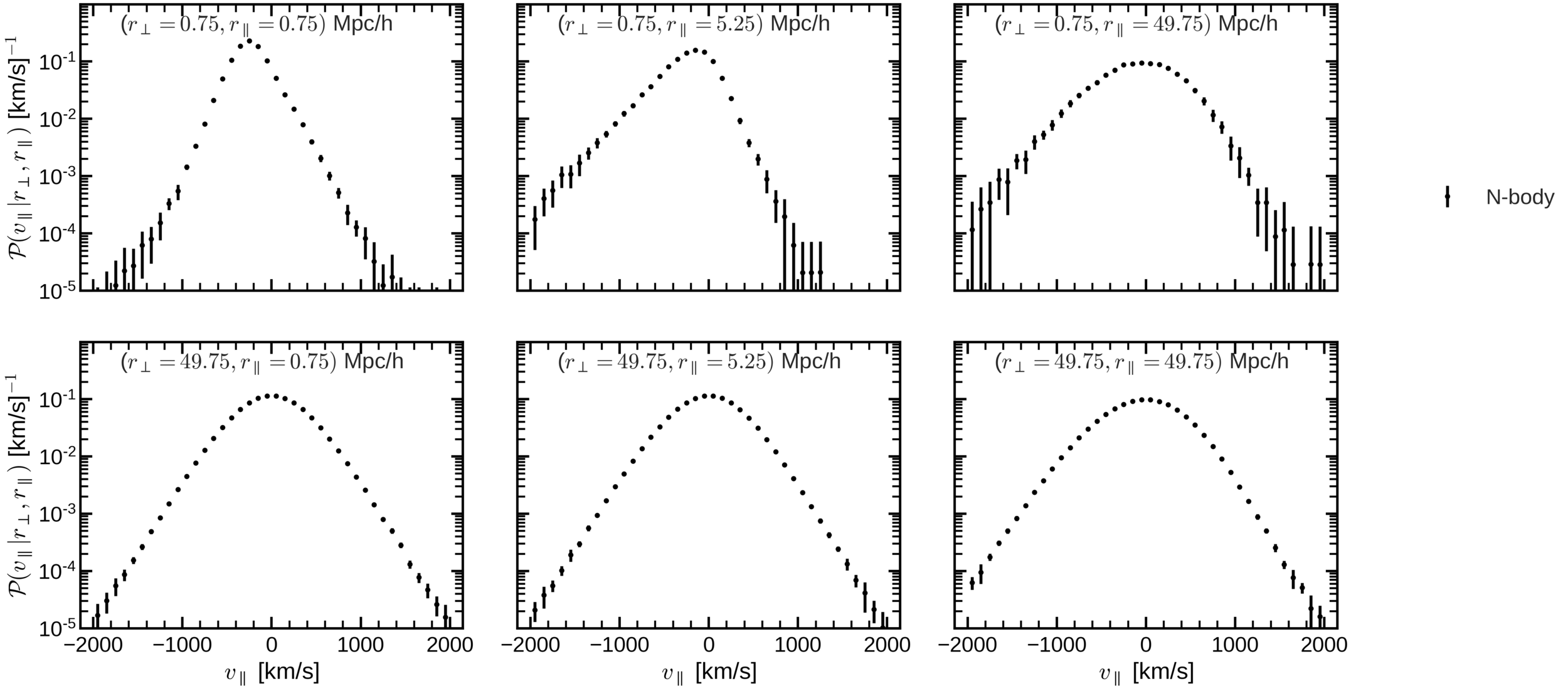
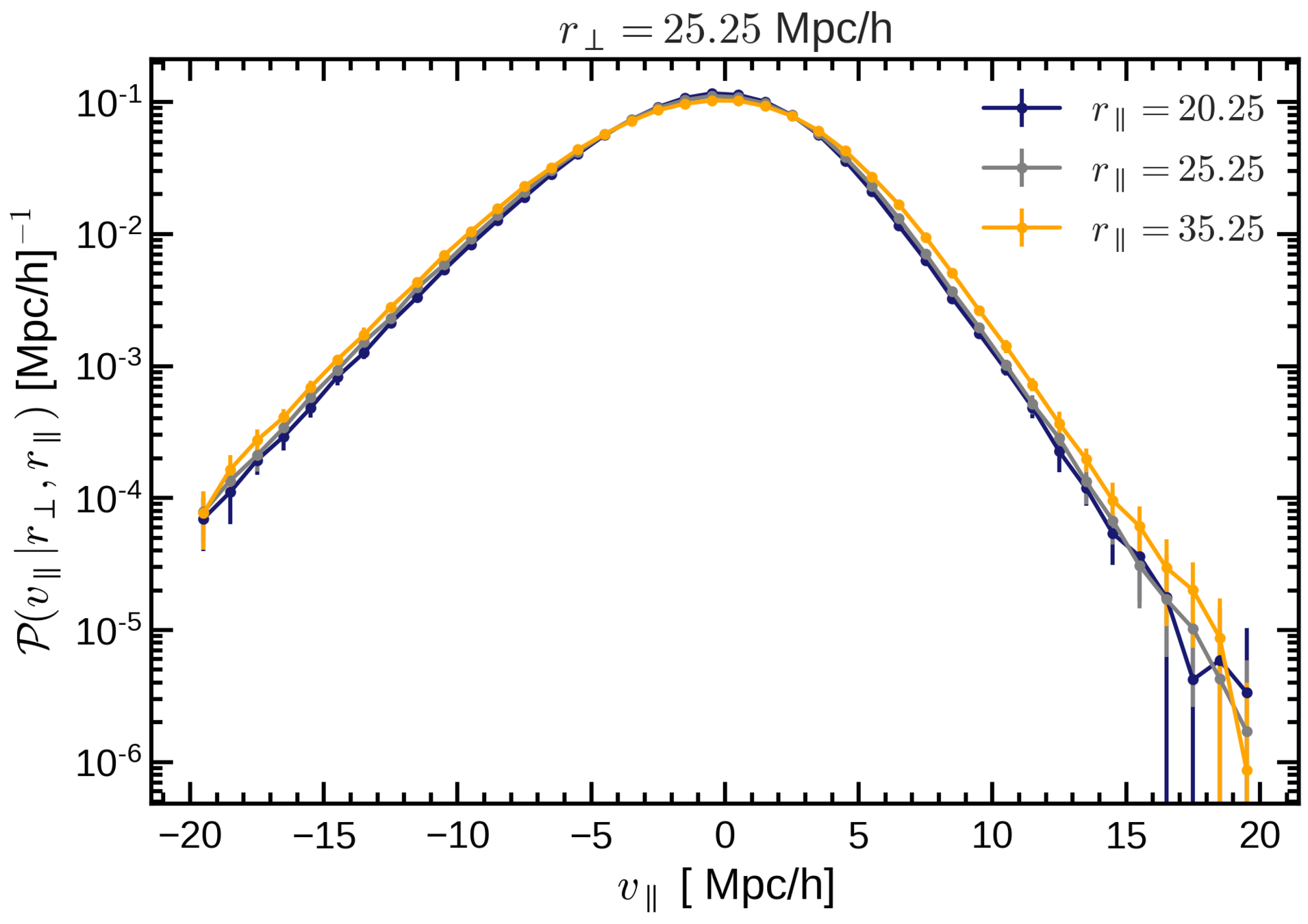
PAIRWISE VELOCITY
DISTRIBUTION
r
v_{\parallel,1}
v_{\parallel,2}
v_{\parallel} = v_{\parallel,1} - v_{\parallel,2}
s
s_{\parallel} = v_{\parallel} + r_{\parallel}
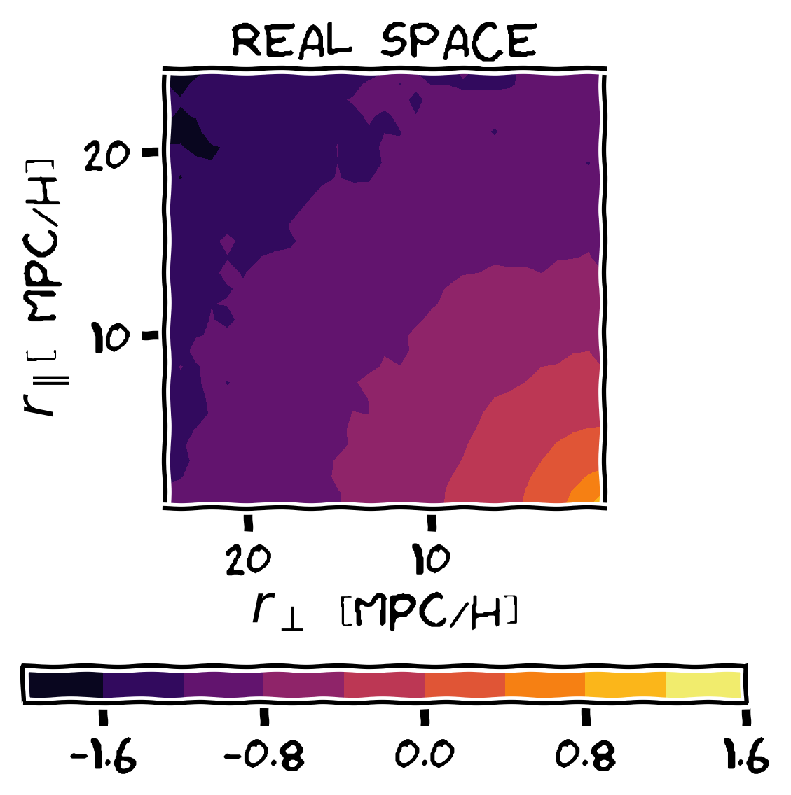
\xi(r)
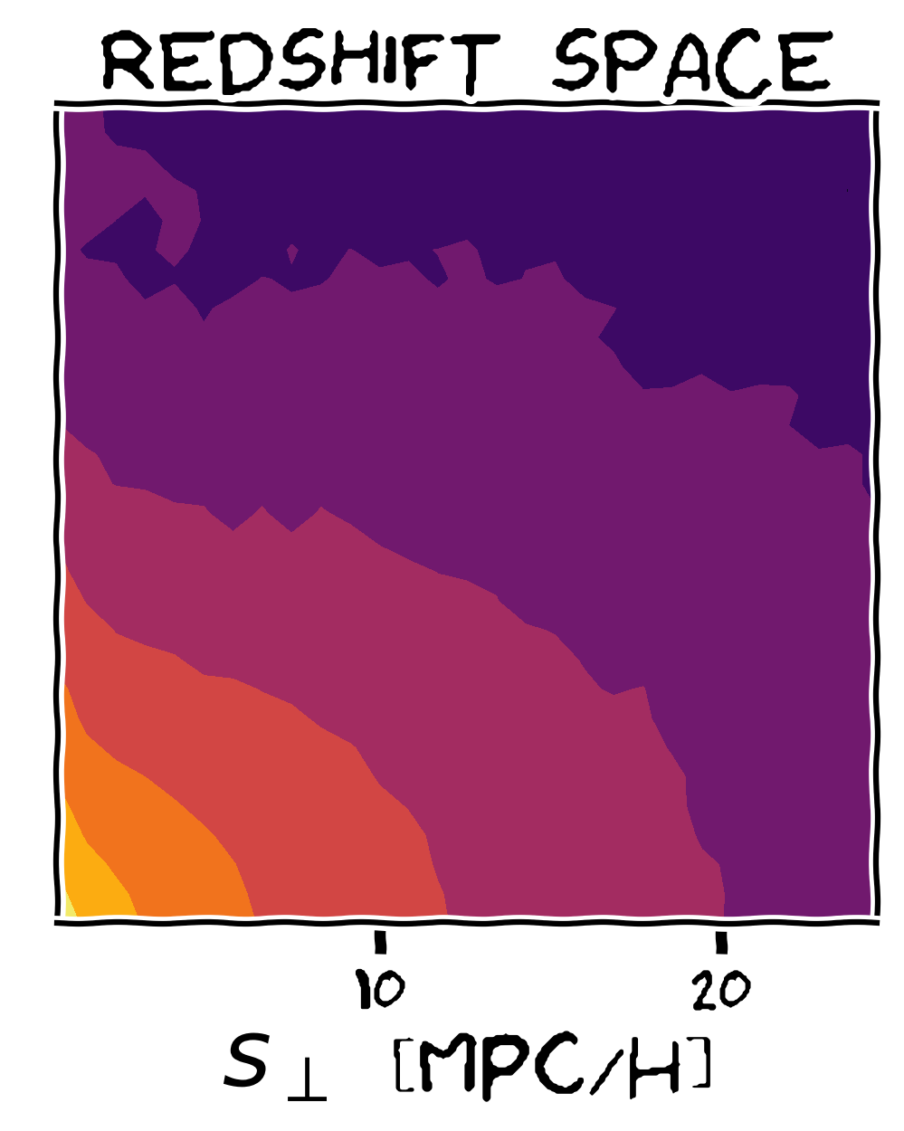
\xi(s_\perp, s_\parallel)
Probability of finding a pair of galaxies at distance r
Virial motions within halos
v_{\parallel,1}
v_{\parallel,2}
Infall towards halos
v_{\parallel,1}
v_{\parallel,2}
\mathrm{Dark \, matter \, halos \, with } \, M > 10^{13} M_\odot
Generating skewness by using the Cummulative distribution
\mathrm{Skewed} = \mathrm{PDF}(v) \mathrm{CDF}[w(v)]
Azzalini Capitanio '09
Symmetric
Odd function
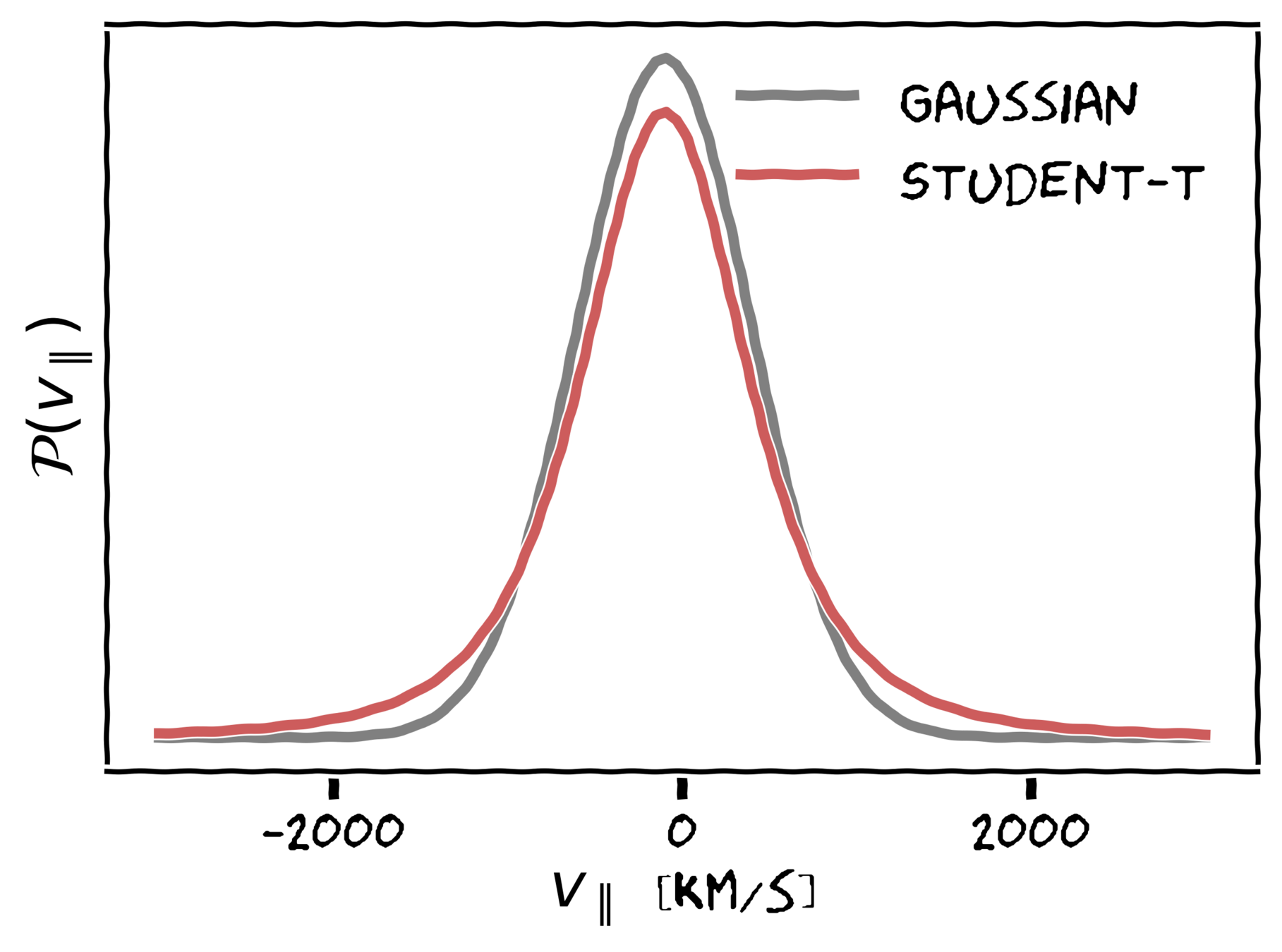
Zu Weinberg '13
Mean
Variance
Skewness
Kurtosis
= 4 free parameters
1+\xi(s_\perp, s_\parallel) = \int d r_\parallel \left(1 + \xi(r)\right )\mathcal{P}(v_\parallel | r_\perp, r_\parallel)
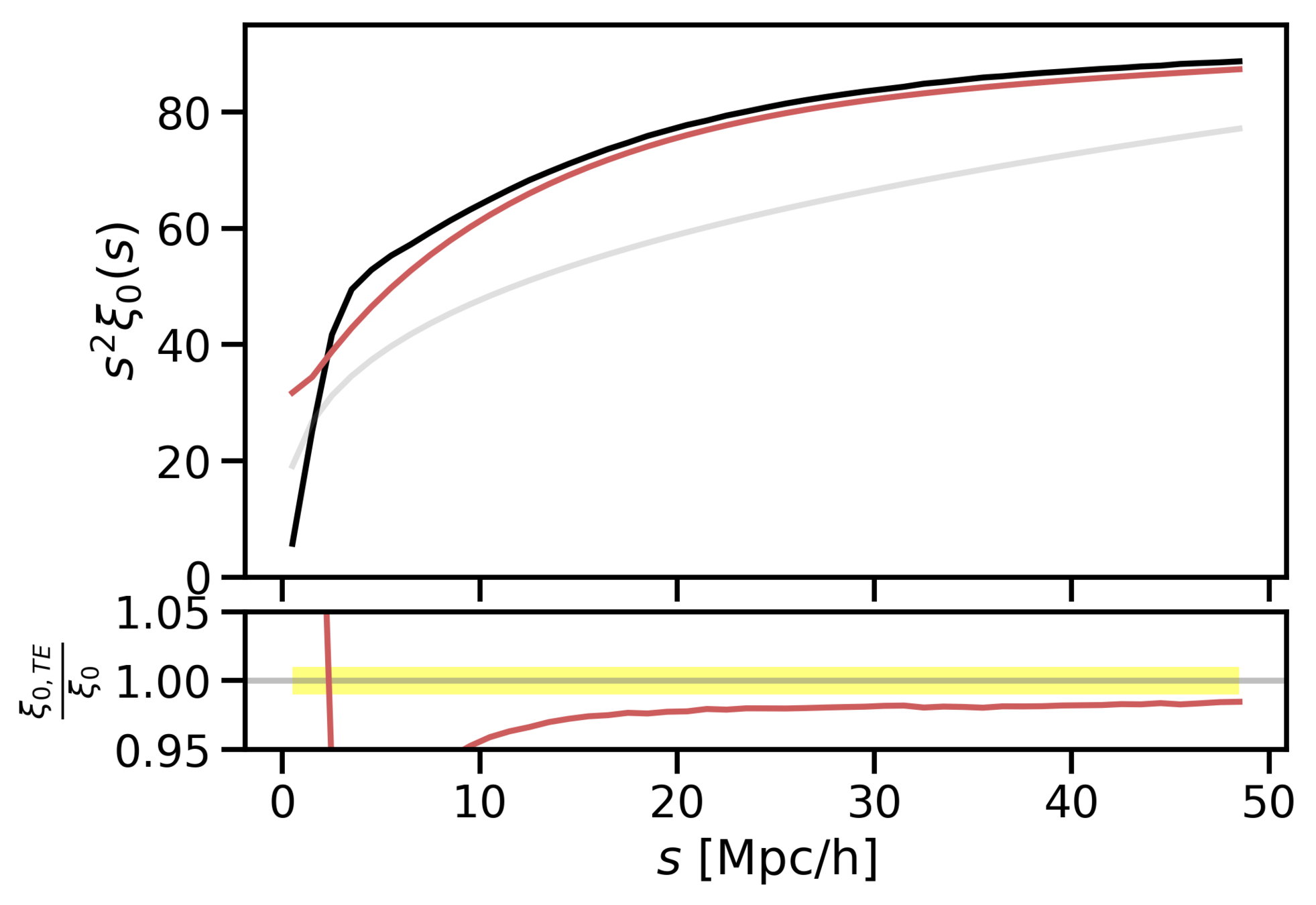
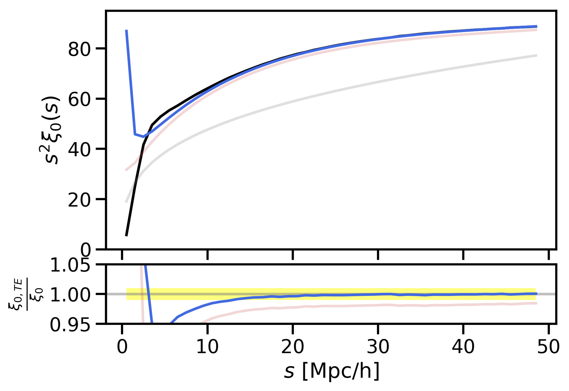
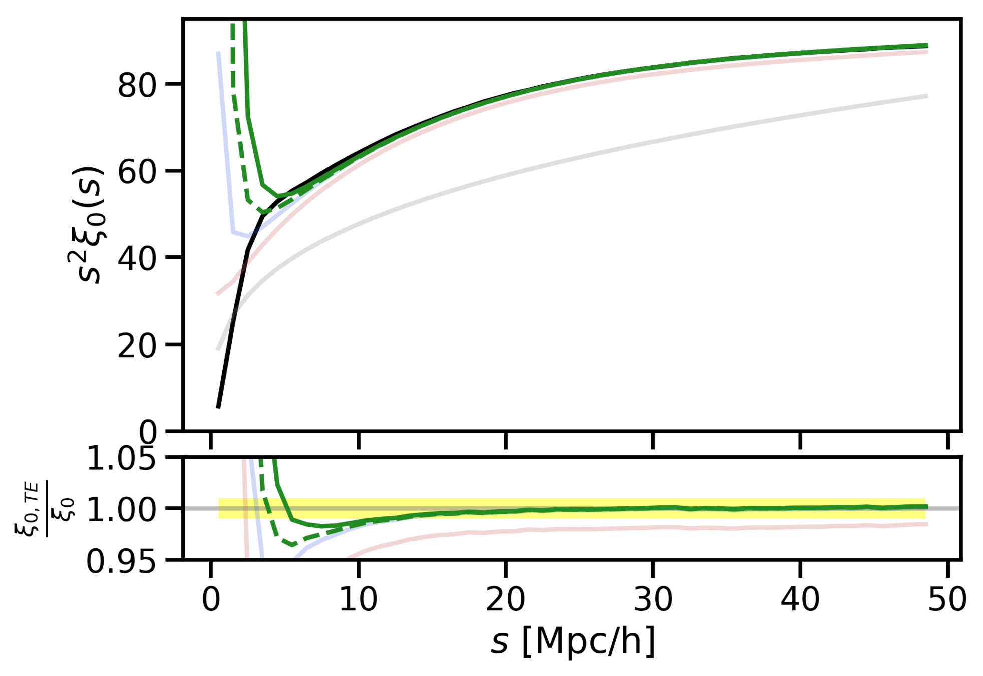
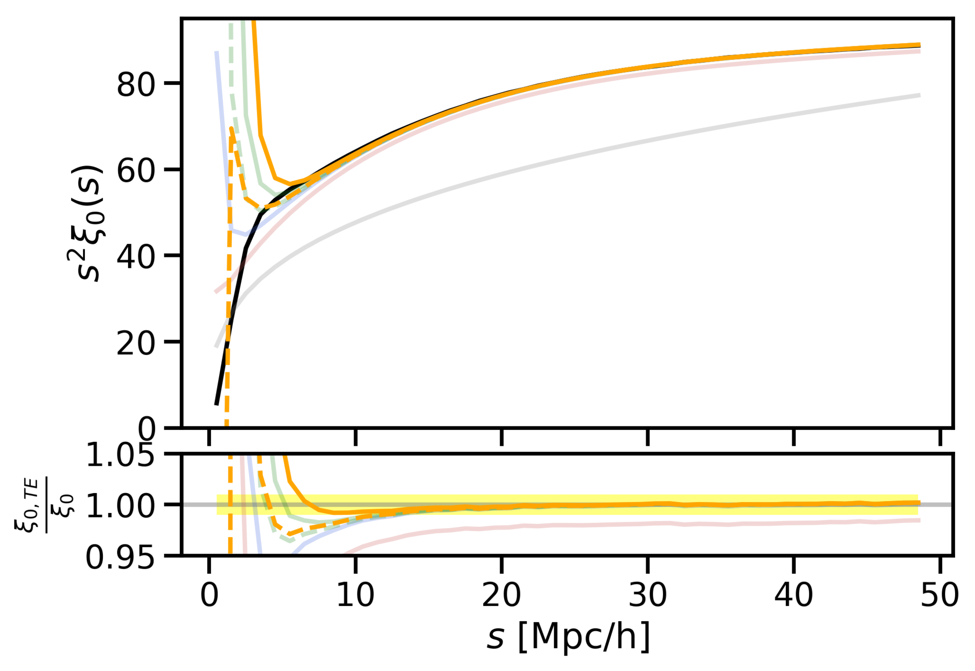
\xi_0 = \int d\mu \, \xi(s, \mu)
s
\mu
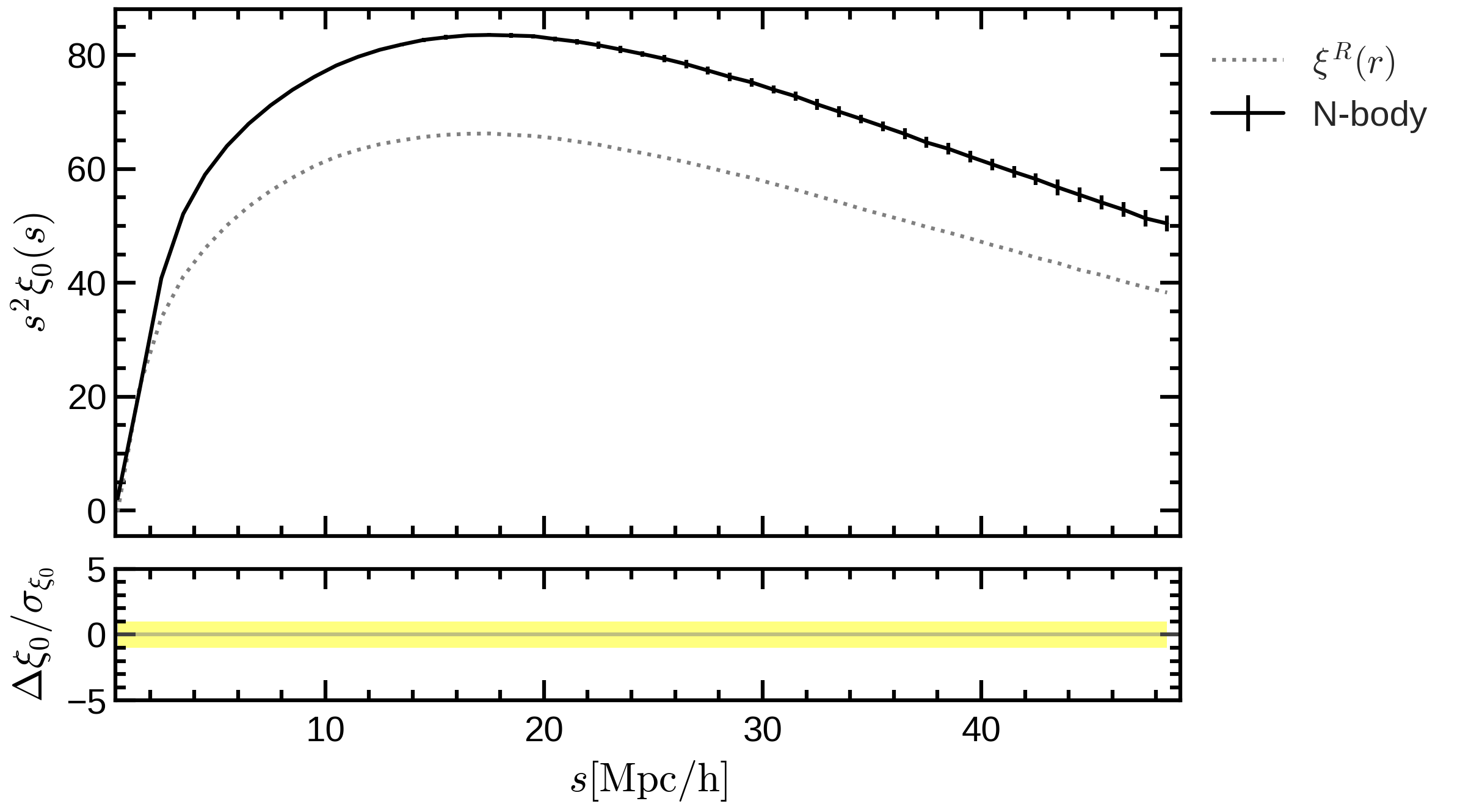
s
\mu
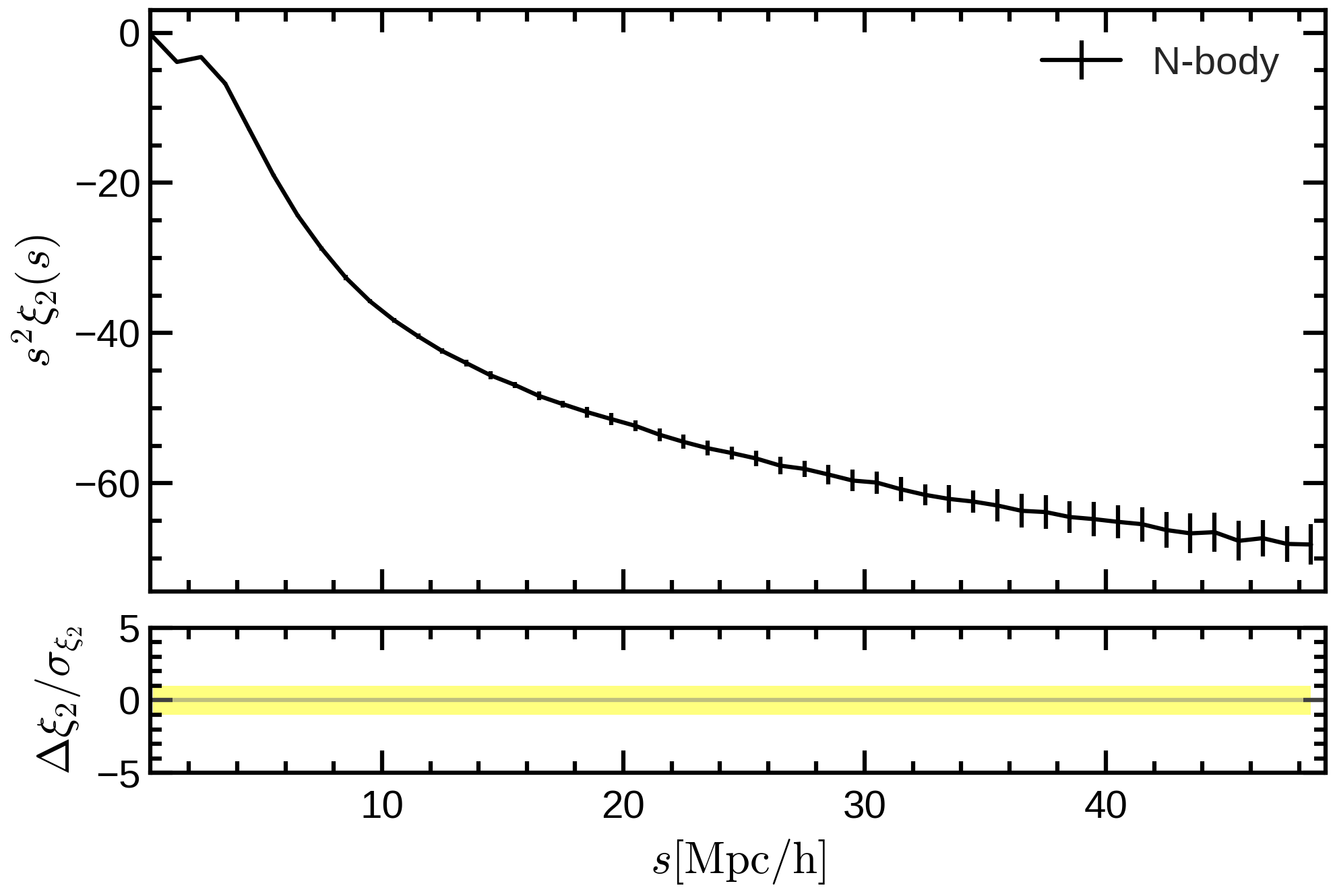
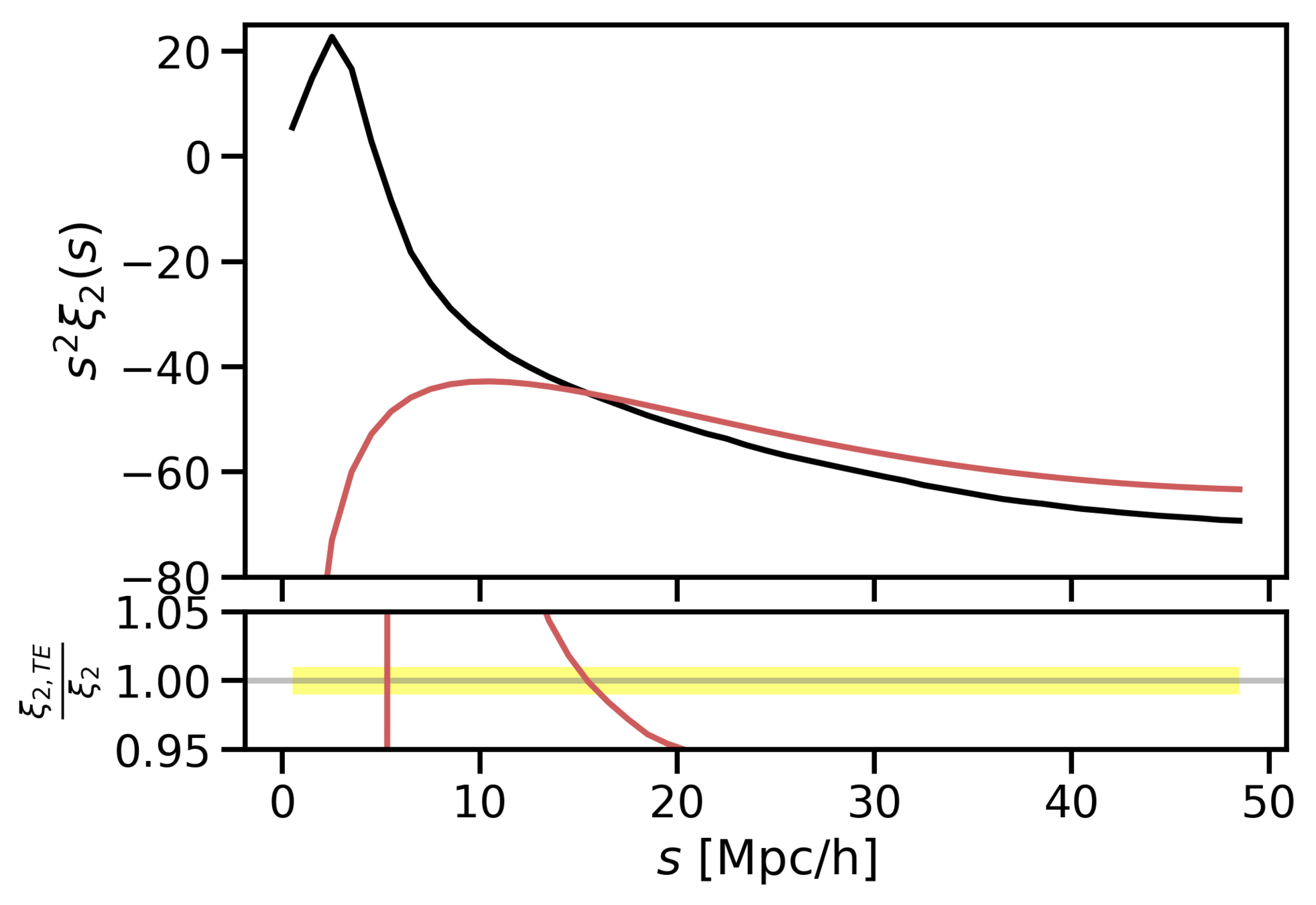
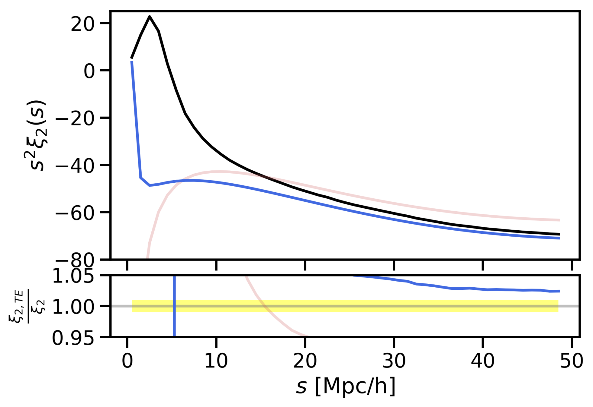
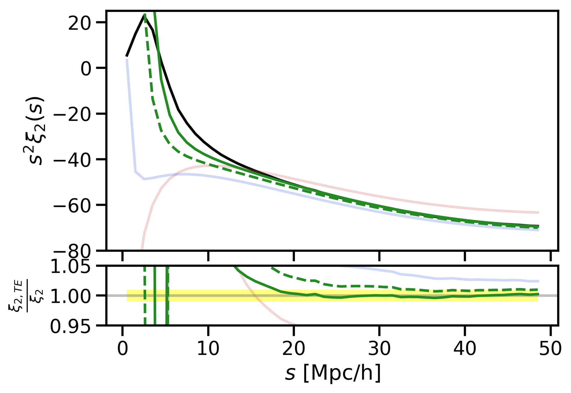
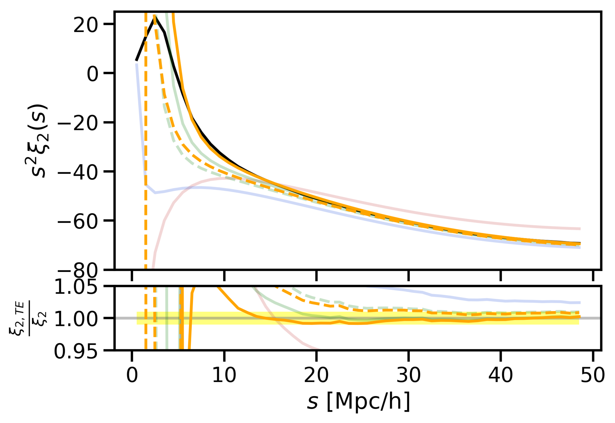
\xi_2 = \frac{1}{2} \int d\mu \,(3\mu^2 - 1) \xi(s, \mu)
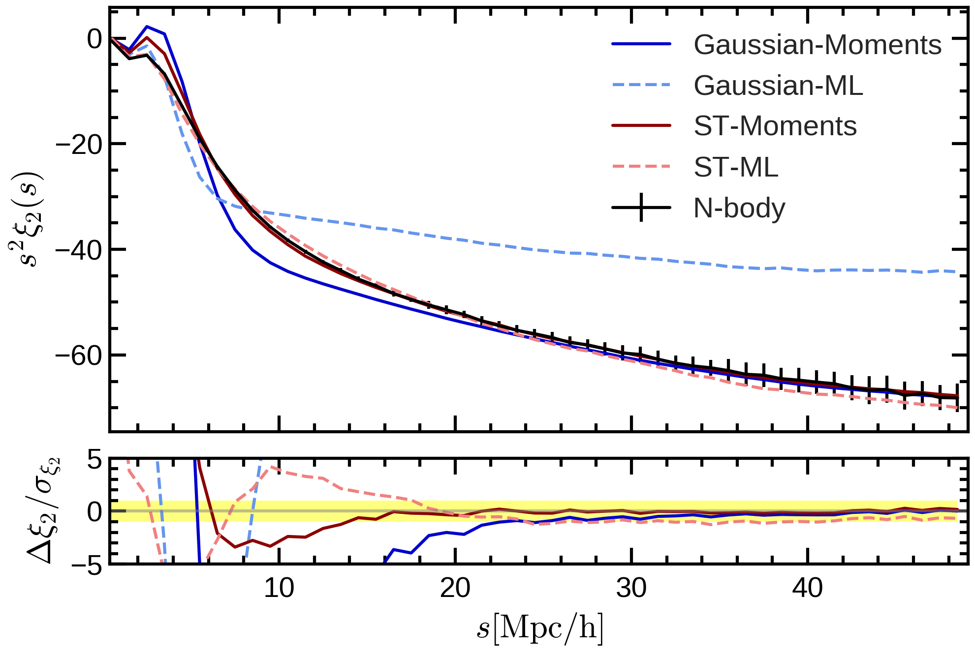
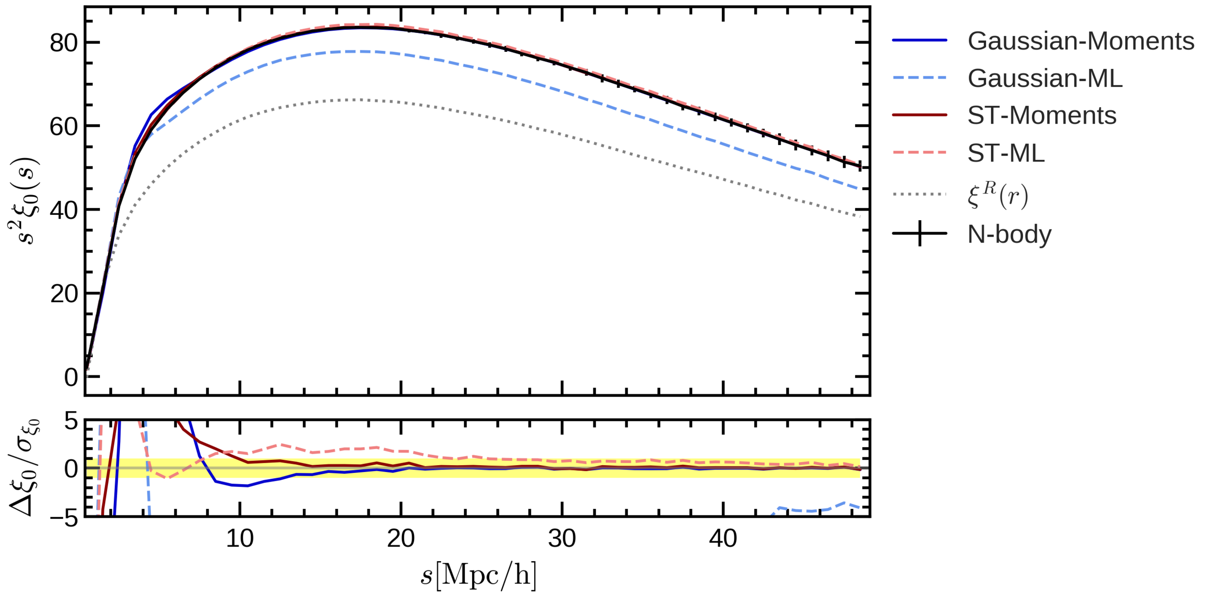
Conclusions
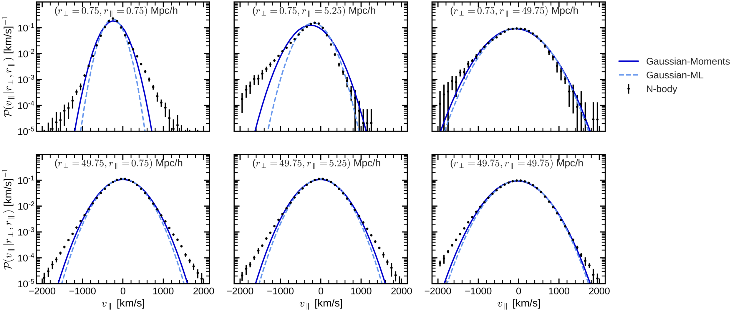
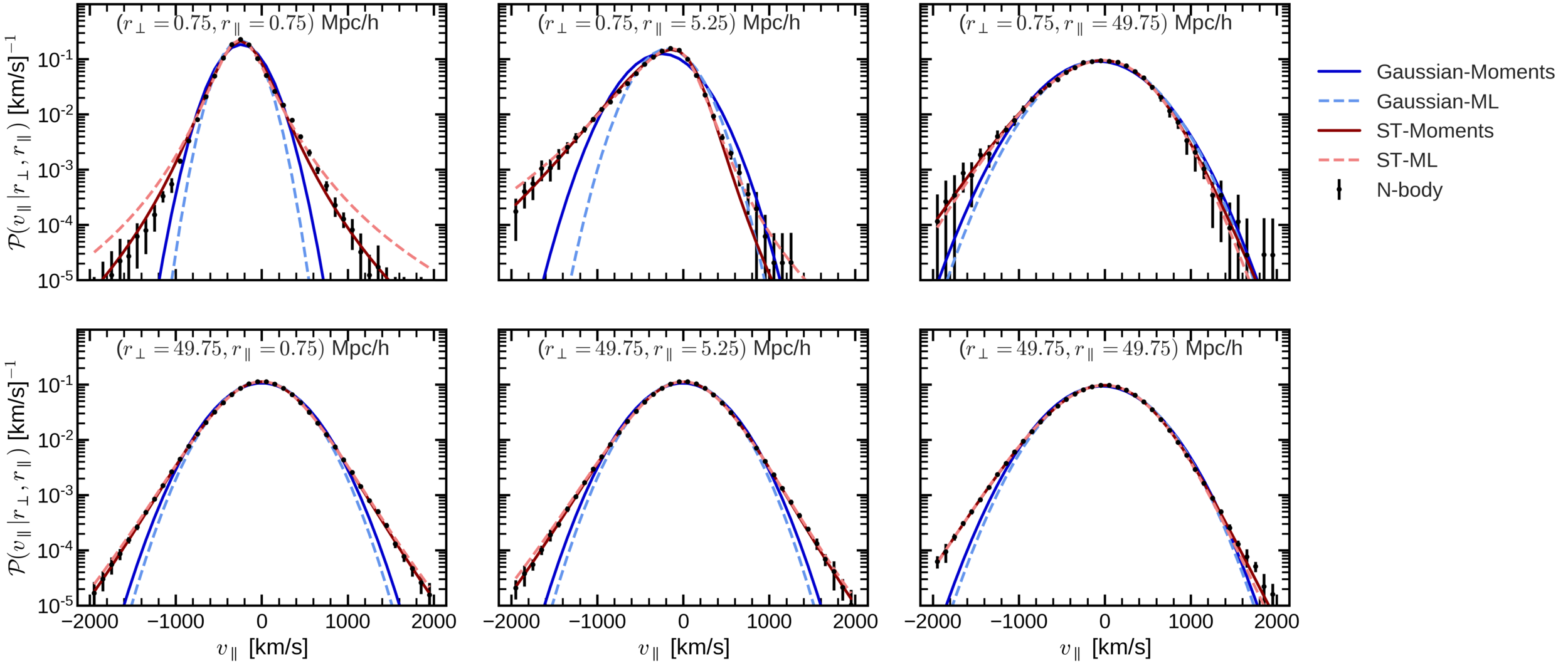
- We have found an accurate mapping (up to 10 Mpc/h) from redshift to real space by adding skewness and kurtosis to the pairwise velocity distribution.
- But, how much does this improve our estimate of the growth factor? -> Next step
- The Gaussian model works well up to intermidiate scales (around 40 Mpc/h), because it has the right first two moments: mean and variance.
Streaming Model of Redshift Space Distortions
1+\xi(s_\perp, s_\parallel) = \int dr_\parallel \left(1 + \xi(r)\right) \mathcal{P}(v_\parallel=s_\parallel-r_\parallel|r_\perp, r_\parallel)
PAIRWISE VELOCITY
DISTRIBUTION
r
v_{\parallel,1}
v_{\parallel,2}
v_{\parallel} = v_{\parallel,1} - v_{\parallel,2}
s
s_{\parallel} = v_{\parallel} + r_{\parallel}
1+\xi(s_\perp, s_\parallel) = \int d r_\parallel \left(1 + \xi(r)\right )\mathcal{P}(v_\parallel | r_\perp, r_\parallel)
\xi_0 = \int d\mu \, \xi(s, \mu)
s
\mu
s
\mu
\xi_2 = \frac{1}{2} \int d\mu \,(3\mu^2 - 1) \xi(s, \mu)
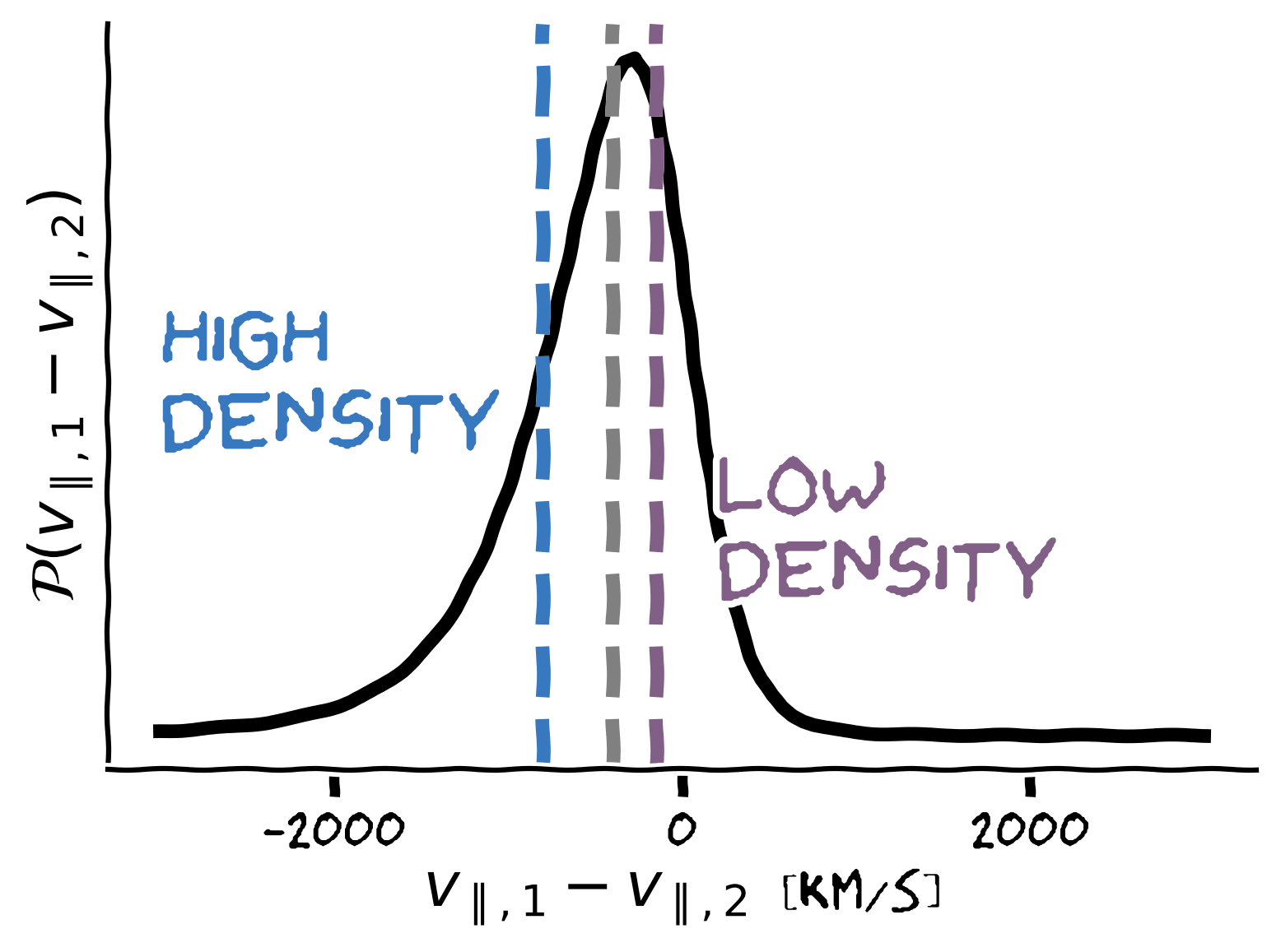
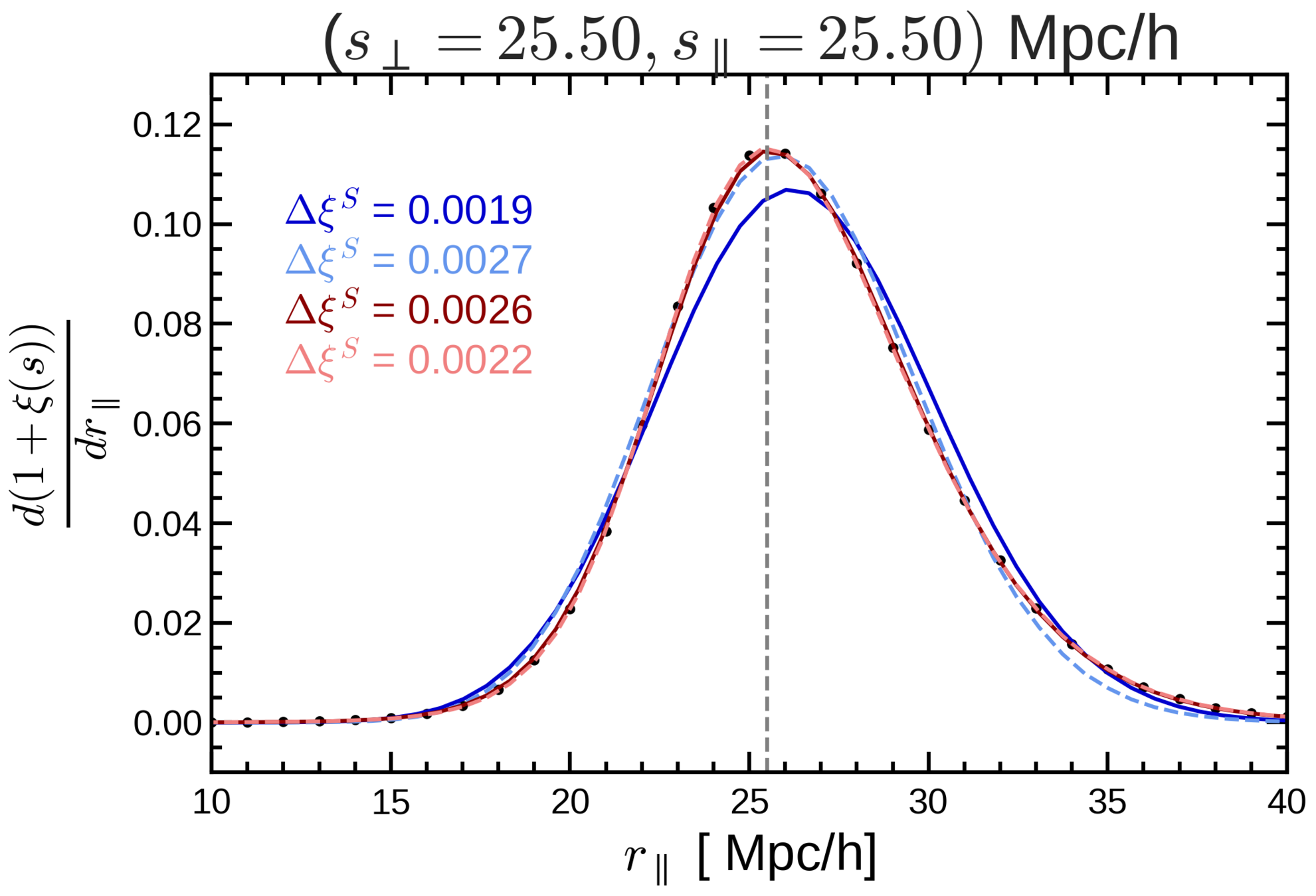
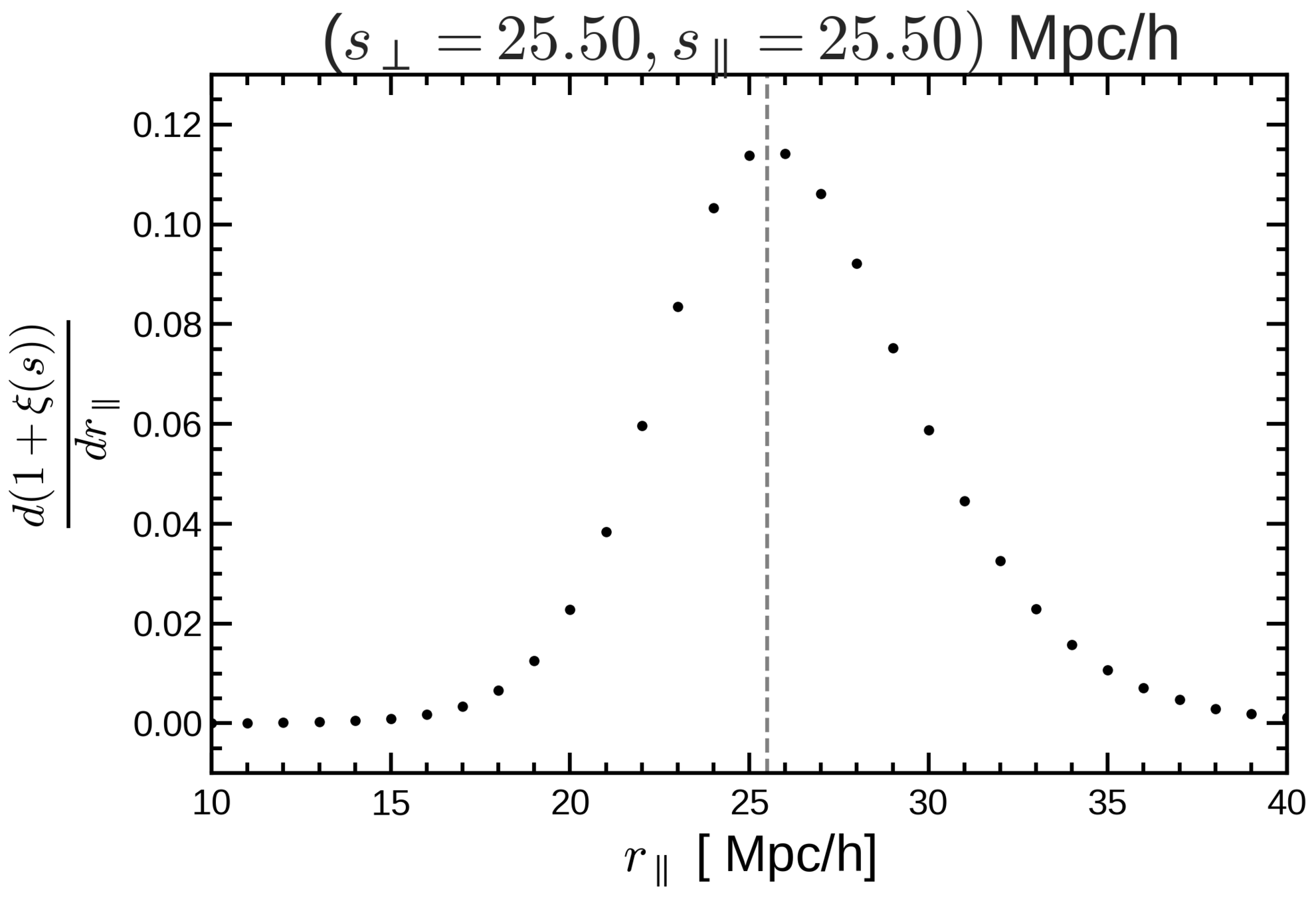
Why does Gaussianity work so well?
\left(1 + \xi(r)\right) \mathcal{P}(v_\parallel=s_\parallel - r_\parallel | r_\perp, r_\parallel)
Peaks at
goes quickly to 0
r_\parallel \approx 0 \rightarrow r \approx s_\perp
Peaks at
r_\parallel \approx s_\parallel
\int dr_\parallel
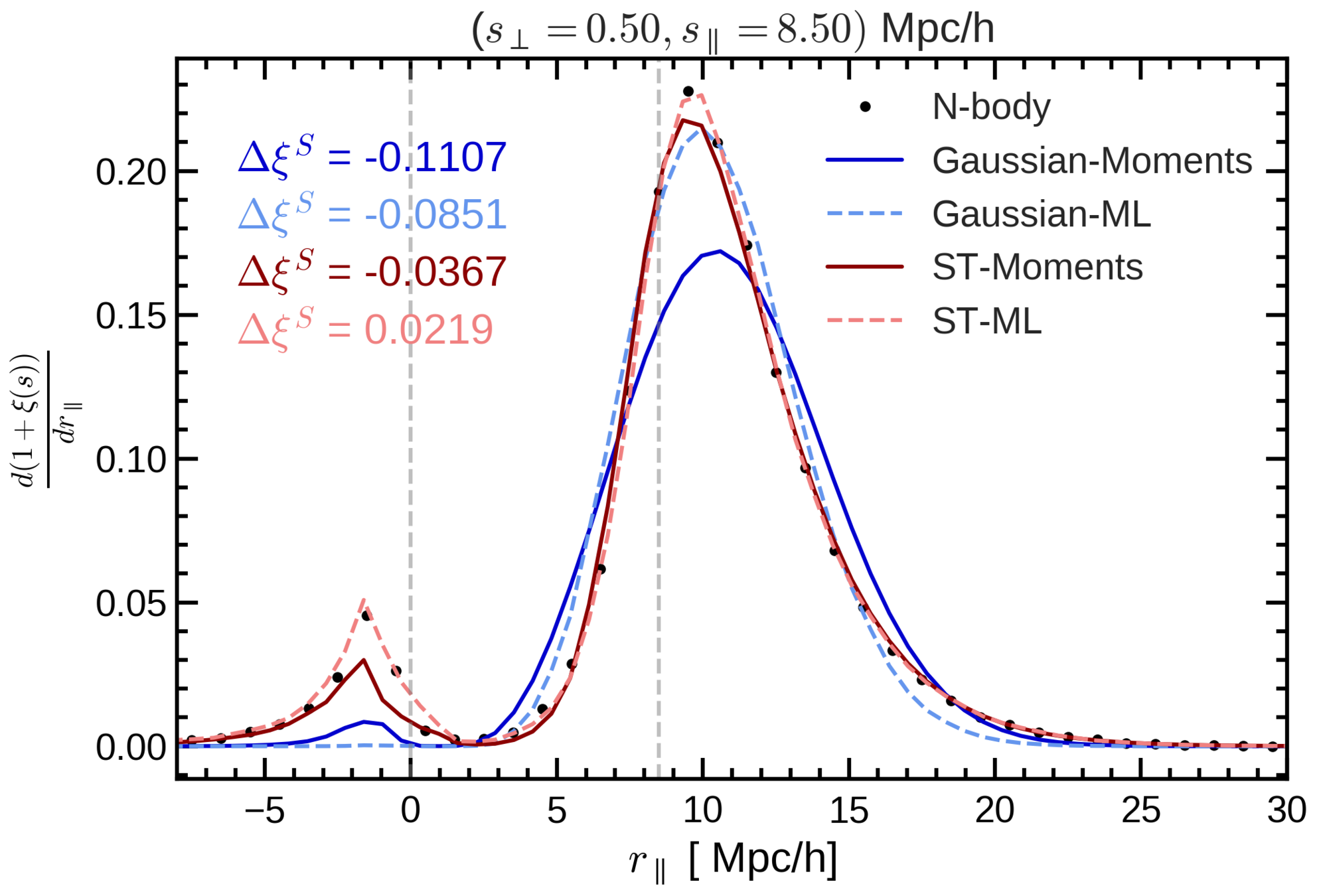
\left(1 + \xi(r)\right) \mathcal{P}(v_\parallel=s_\parallel - r_\parallel | r_\perp, r_\parallel)
Why does Gaussianity work so well?
\left(1 + \xi(r)\right) \mathcal{P}(v_\parallel=s_\parallel - r_\parallel | r_\perp, r_\parallel)
r_\parallel = s_\parallel
\mathrm{Taylor \, expand } \, \mathcal{P}(v_\parallel | r_\perp, r_\parallel)\, \mathrm{around} \, r_\parallel=s_\parallel
Taylor expansion
\xi^S (s_\perp, s_\parallel) \approx
\xi^R(s)
- \frac{d m_1}{d s_\parallel}
+ \frac{1}{2} \frac{d^2 m_2}{d s_\parallel^2}
- \frac{1}{3} \frac{d^3 m_3}{d s_\parallel^3}
+ \frac{1}{4} \frac{d^4 m_4}{d s_\parallel^4}
SKEWNESS (c3)
KURTOSIS
m_3 = (c_3) + 3 m_1 m_2 + 2 m_1^3
Gaussian
(c3=0)
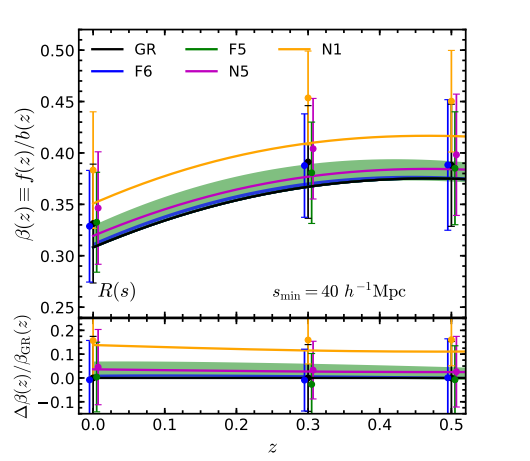
Growth rate might be different on
different scales
Growth of strcuture
Redshift
Edinburgh_2020
By carol cuesta


