


Charles Gunn
Mathemagician, 3D developer, geometer, geometric algebra aficionado, mathematics moviemaker, father, gardener ...
Projective Geometric Algebra:
A Swiss army knife for doing
Cayley-Klein geometry
Charles Gunn
Sept. 18, 2019 at ICERM, Providence
Full-featured slides available at: https://slides.com/charlesgunn3/icerm2019.
Check for updates incorporating new ideas inspired by giving the talk.
This first slide will indicate whether update has occurred.
SIGNATURE of Quadratic Form
Example: \((++-0) = (2,1,1)\)
\(~e_0\cdot e_0 = e_1\cdot e_1 = +1,~e_2\cdot e_2=-1,~e_3\cdot e_3=0,\)\(~~e_i\cdot e_j = 0 ~\text{for}~i\neq j\)
| Signature of Q | Space | Symbol | |
|---|---|---|---|
| +1 | elliptic | ||
| -1 | hyperbolic | ||
| 0 | euclidean |
\((n+1,0,0)\)
$$\bf{E}^n$$
$$\bf{H}^n$$
$$\bf{Ell}^n,\bf{S}^n$$
\((n,1,0)\)
\("(n,0,1)"\)
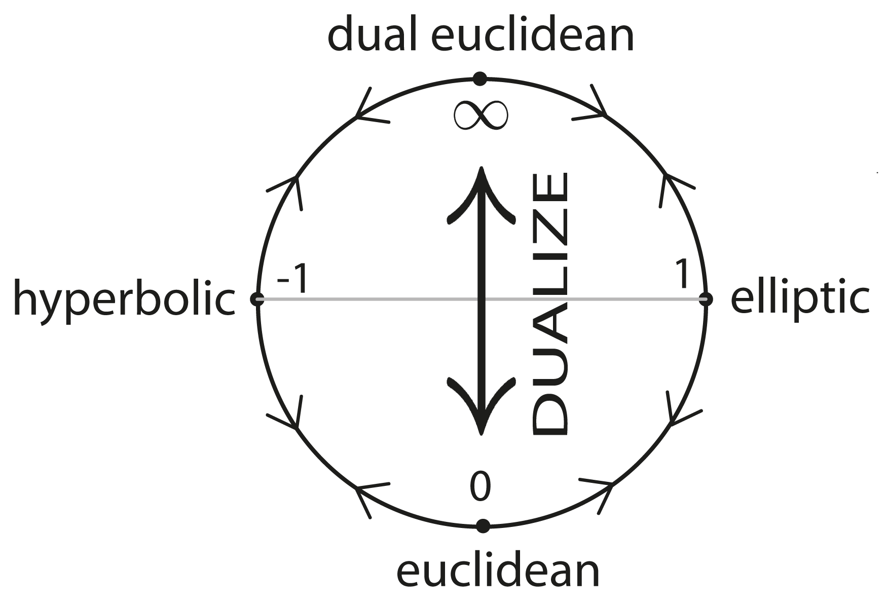
\(\kappa\)
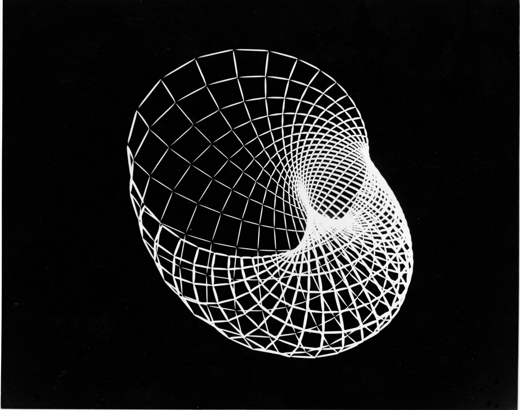
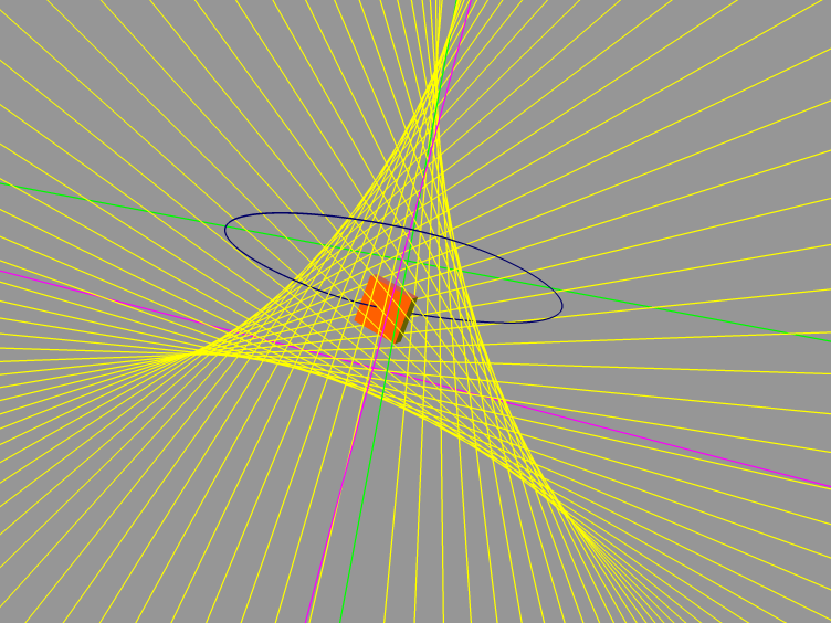
The Sudanese Moebius band in \(S^3\) discovered by Sue Goodman and Dan Asimov, visualized in UNC-CH Graphics Lab, 1979.
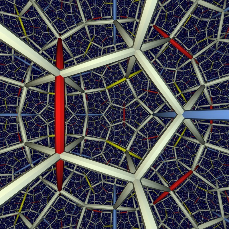
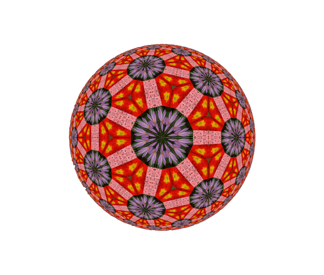
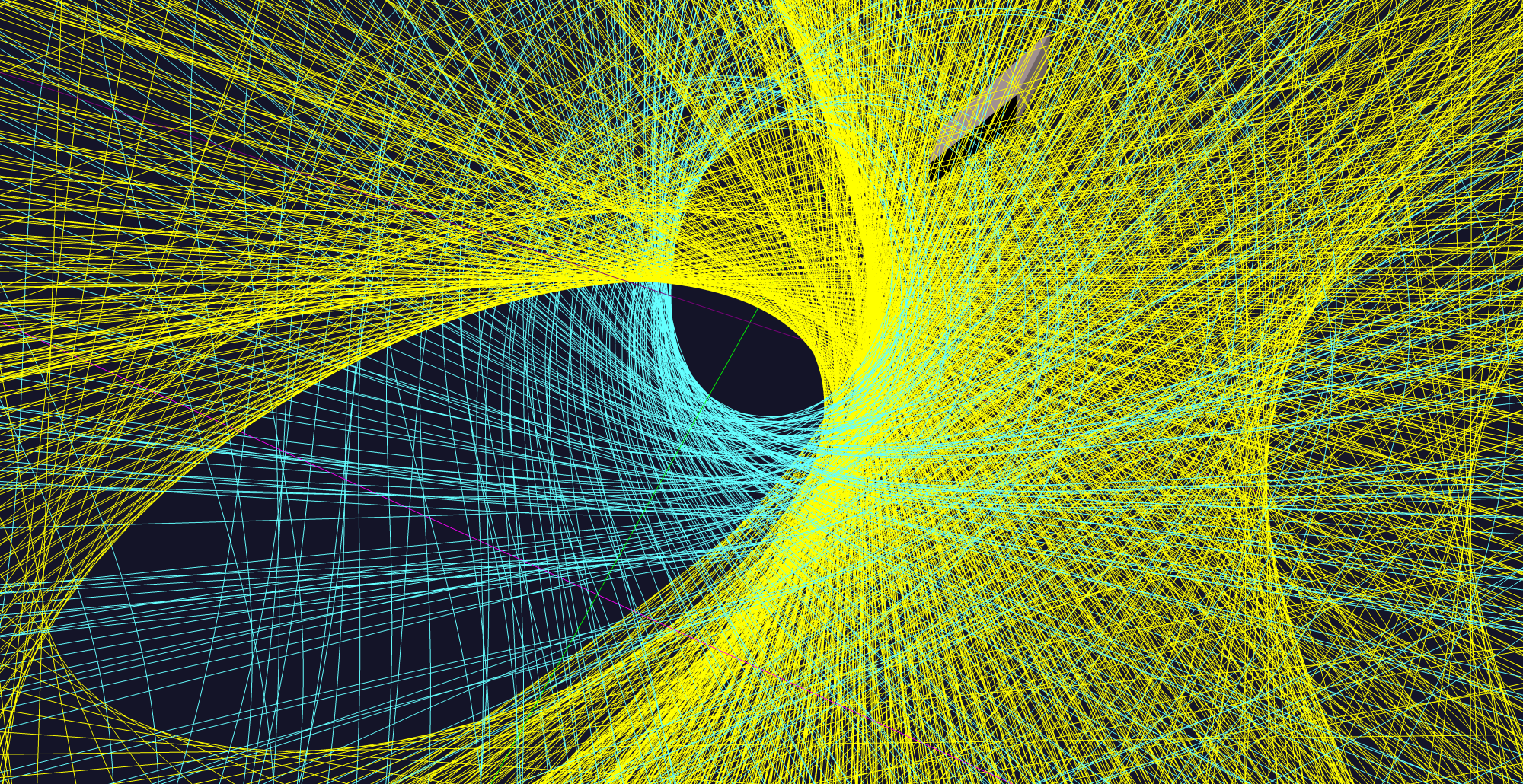
Tessellation of \(H^3\) with regular right-angled dodecahedra (from "Not Knot", Geometry Center, 1993).
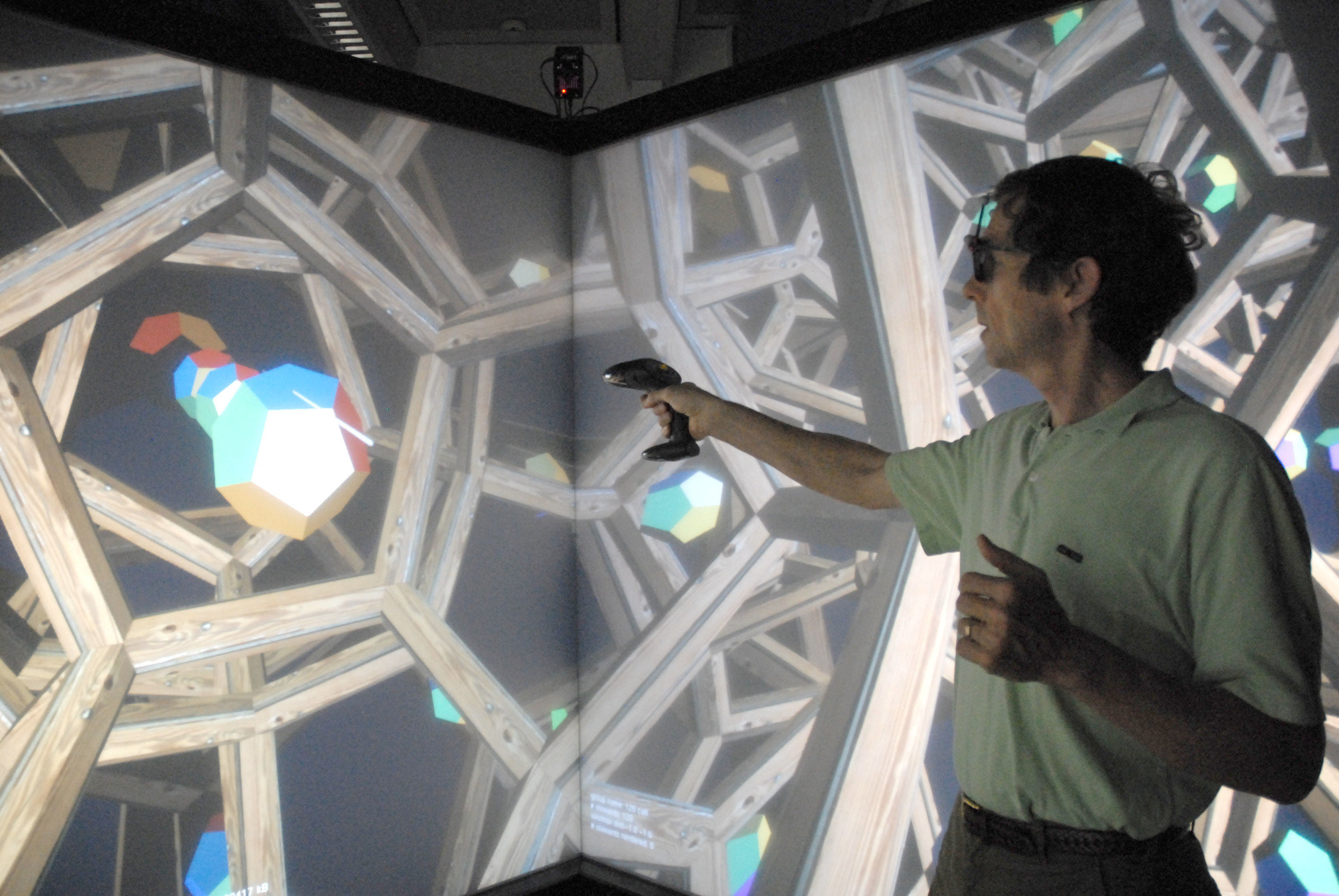
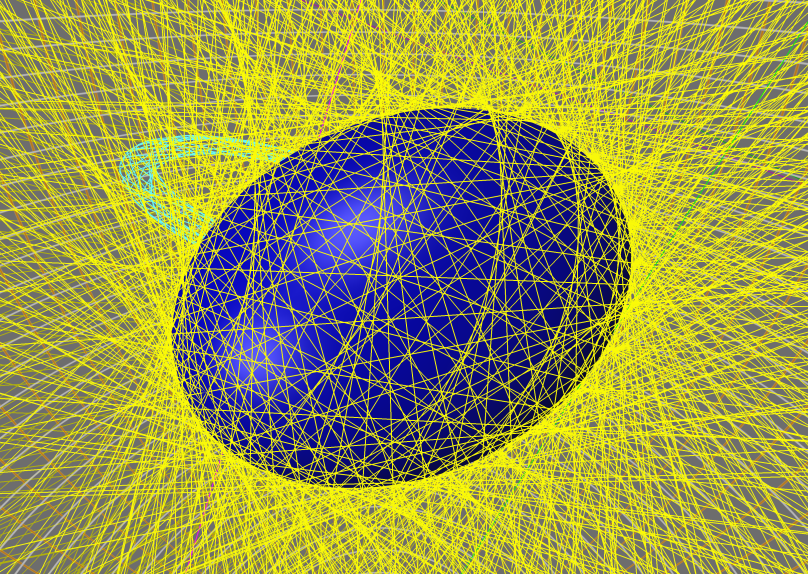
The 120-cell, a tessellation of the 3-sphere \(\bf{S}^3\)
(PORTAL VR, TU-Berlin, 18.09.09)
| Name | elliptic | euclidean | hyperbolic |
|---|---|---|---|
| signature | (3,0,0) | "(2,0,1)" | (2,1,0) |
| null points |
\(x^2+y^2+z^2\)=0
\(z^2\)=0
\(x^2+y^2-z^2\)=0
| Name | elliptic | euclidean | hyperbolic |
|---|---|---|---|
| signature | (3,0,0) | "(2,0,1)" | (2,1,0) |
| null points | |||
| null lines* |
\(x^2+y^2+z^2\)=0
\(z^2\)=0
\(x^2+y^2-z^2\)=0
\(a^2+b^2+c^2\)=0
\(a^2+b^2-c^2\)=0
\(a^2+b^2\)=0
*The line \(ax+by+cz=0\) has line coordinates \((a,b,c)\).
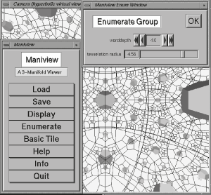
1993
2019
Projective
points
Projective
matrices
Projective
points
Projective
matrices
But it's 2019 now. Can we do better?
Coordinate-free
Uniform rep'n for points, lines, and planes
Single, uniform rep'n for isometries
Parallel-safe meet and join operators
Compact expressions for classical geometric results
Physics-ready
Metric-neutral
Backwards compatible
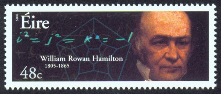
A 4D algebra generated by units \(\{1,\mathbf{i},\mathbf{j},\mathbf{k}\}\) satisfying:
$$1^2=1,~~\mathbf{i}^2=\mathbf{j}^2=\mathbf{k}^2=-1$$ $$\mathbf{i}\mathbf{j}=-\mathbf{j}\mathbf{i},\text{...}$$
Quaternions \(\mathbb{H}\)
Im. quaternions \(\mathbb{IH}\)
Unit quaternions \(\mathbb{U} \)
$$s+x\mathbf{i}+y\mathbf{j}+z\mathbf{k}$$
$$ \mathbf{v} := x\mathbf{i}+y\mathbf{j}+z\mathbf{k} \Leftrightarrow (x,y,z) \in \mathbb{R}^3 $$
$$\{\mathbf{g}\in\mathbb{H} \mid \mathbf{g}\overline{\mathbf{g}}= 1\}$$
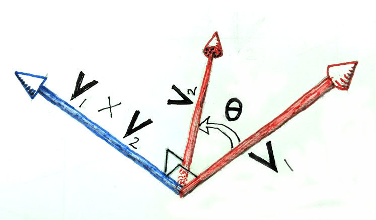
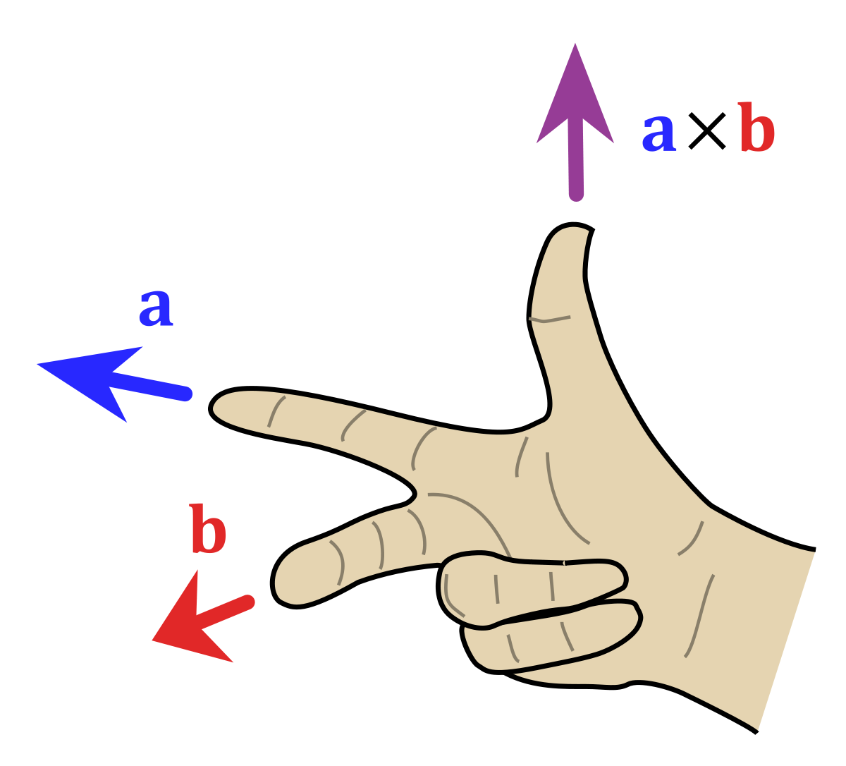
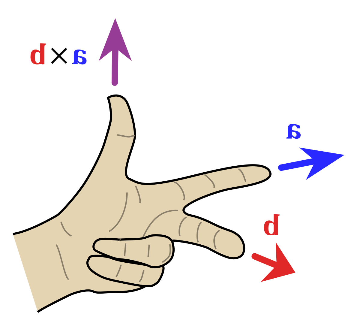
I. Geometric product:
$$\mathbf{v}_1\mathbf{v}_2 = -\mathbf{v}_1 \cdot \mathbf{v}_2 + \mathbf{v}_1 \times \mathbf{v}_2$$
cross product
inner product
Quaternions \(\mathbb{H}\)
Im. quaternions \(\mathbb{IH}\)
Unit quaternions \(\mathbb{U} \)
$$s+x\mathbf{i}+y\mathbf{j}+z\mathbf{k}$$
$$ \mathbf{v} := x\mathbf{i}+y\mathbf{j}+z\mathbf{k} \Leftrightarrow (x,y,z) \in \mathbb{R}^3 $$
$$\{\mathbf{g}\in\mathbb{H} \mid \mathbf{g}\overline{\mathbf{g}}= 1\}$$
II. Rotations via sandwiches:
1. For \(\mathbf{g} \in \mathbb{U}\), there exists \(\mathbf{x} \in \mathbb{IH}\) so that
$$\mathbf{g} = \cos(t)+\sin(t)\mathbf{x} = e^{t\mathbf{x}}$$
2. For any \(\mathbf{v} \in \mathbb{IH}~~ (\cong \mathbb{R}^3)\), the "sandwich" $$ \mathbf{g}\mathbf{v}\overline\mathbf{g}$$ rotates \(\mathbf{v}\) around the axis \(\mathbf{x}\) by an angle \(2t\).
3. Comparison to matrices.
Quaternions \(\mathbb{H}\)
Im. quaternions \(\mathbb{IH}\)
Unit quaternions \(\mathbb{U} \)
$$s+x\mathbf{i}+y\mathbf{j}+z\mathbf{k}$$
$$ \mathbf{v} := x\mathbf{i}+y\mathbf{j}+z\mathbf{k} \Leftrightarrow (x,y,z) \in \mathbb{R}^3 $$
$$\{\mathbf{g}\in\mathbb{H} \mid \mathbf{g}\overline{\mathbf{g}}= 1\}$$
I. Geometric product
II. Rotations as sandwiches
I. Only applies to points/vectors
II. Special case \(\mathbb{R}^3\)
Hermann Grassmann (1809-1877)
Ausdehnungslehre (1844)
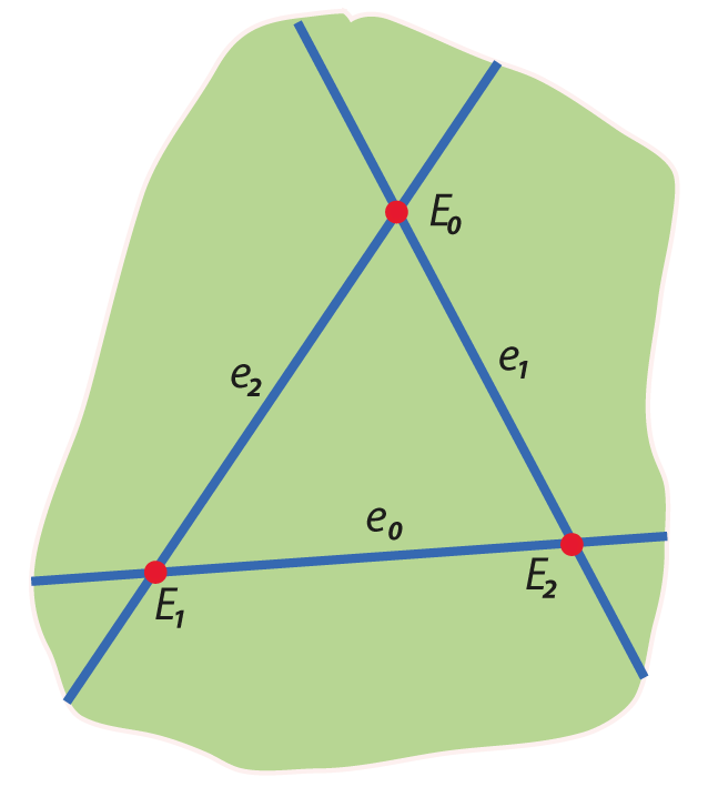
The wedge (\(\wedge\)) product in \(\mathbb{R}P^2\) and \(\mathbb{R}P^{2\large*}\)
Standard projective
\(\mathbf{x}\wedge\mathbf{y}\) is join
yields \(\bigwedge\mathbb{R}P^2\)
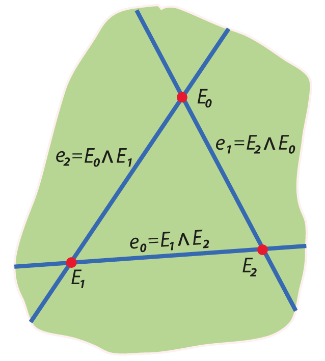
Dual projective
\(\mathbf{x}\wedge\mathbf{y}\) is meet
yields \(\bigwedge\mathbb{R}P^{2\large*}\)
| Grade | Sym | Generators | Dim. | Type |
|---|---|---|---|---|
| 0 | 1 | 1 | Scalar | |
| 1 | 3 | Line | ||
| 2 | 3 | Point | ||
| 3 | 1 | Pseudoscalar |
\(\bigwedge^3\)
\(\bigwedge^2\)
\(\bigwedge^1\)
\(\bigwedge^0\)
\(\{\mathbf{e}_0,\mathbf{e}_1,\mathbf{e}_2\}\)
\(\{\mathbf{E}_i = \mathbf{e}_j\wedge\mathbf{e}_k\}\)
\(\mathbf{I}=\mathbf{e}_0\wedge\mathbf{e}_1\wedge\mathbf{e}_2\)
We will be using \(\bigwedge\mathbb{R}P^{n\large{*}}\) for the rest of the talk.
The dual projective Grassmann algebra \(\bigwedge\mathbb{R}P^{2\large*}\)
Properties of \(\wedge\)
1. Antisymmetric: For 1-vectors \(\mathbf{x}, \mathbf{y}\):$$\mathbf{x}\wedge\mathbf{y}=-\mathbf{y}\wedge\mathbf{x}$$$$\mathbf{x}\wedge\mathbf{x}=0$$
2. Subspace lattice: For linearly independent subspaces \(\mathbf{x}\in\bigwedge^k,\mathbf{y}\in\bigwedge^{m}\), \(\mathbf{x}\wedge\mathbf{y}\in\bigwedge^{k+m}\) is the subspace spanned by \(\mathbf{x}\) and \(\mathbf{y}\) otherwise it's zero.
Note: The regressive (join) product \(\large\vee\) is also available.
(Then it's called a Grassmann-Cayley algebra.)
The wedge (\(\wedge\)) product in \(\mathbb{R}P^2\)
Note: spanning subspace means different things in standard and dual setting. In 3D:
Standard: a line is the subspace spanned by two points.
Dual: a line is the subspace spanned by two planes.
Point range
Spear
Plane pencil
Axis
1. Points, lines, and planes are equal citizens.
2. "Parallel-safe" meet and join operators since projective.
1. Only incidence (projective), no metric.
William Kingdon Clifford (1845-1879)
"Applications of Grassmann's extensive algebra" (1878):
His stated aim: to combine quaternions with Grassmann algebra.
Geometric product extends the wedge product and is defined for two 1-vectors as: $$\large{\mathbf{x}\mathbf{y} := \mathbf{x}\large{\cdot}\mathbf{y} + \mathbf{x}\wedge\mathbf{y}}$$
where \(\cdot\) is the inner product induced by \(\mathbf{Q}\).
0-vector
2-vector
This product can be extended to the whole Grassmann algebra to produce the geometric algebra \(\mathbf{P}(\mathbb{R}^*_{p,n,z})\).
measures sameness
measures difference
Since the two terms measure different aspects, the sum is (usually) non-zero.
We call an algebra constructed in this way a projective geometric algebra (PGA).
We are interested in \(\mathbf{P}(\mathbb{R}^*_{3,0,0}) \), \(\mathbf{P}(\mathbb{R}^*_{2,1,0}) \), \(\mathbf{P}(\mathbb{R}^*_{2,0,1}) \).
We sometimes write \(\mathbf{P}(\mathbb{R}^*_\kappa)\) and leave the metric open.
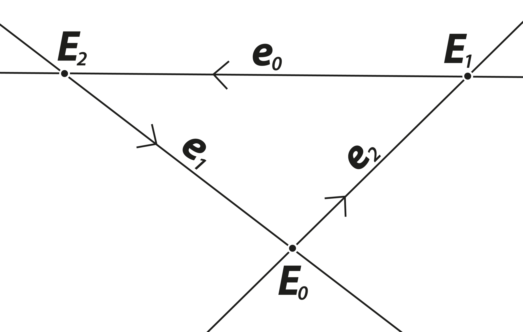
We can choose a fundamental triangle so that:
$$\mathbf{e}_0^2 = \kappa, \mathbf{e}_1^2=\mathbf{e}_2^2=1$$ $$(\kappa\in\{-1,0,1\})$$
$$\mathbf{E}_k:=\mathbf{e}_i\mathbf{e}_j = \mathbf{e}_i\wedge\mathbf{e}_j = -\mathbf{e}_j\mathbf{e}_i$$
$$\mathbf{I}:=\mathbf{e}_0\mathbf{e}_1\mathbf{e}_2$$
Example: Two lines, let \(e_0^2=\kappa\) $$\mathbf{a} = a_0 e_0+a_1 e_1 + a_2 e_2$$ $$ \mathbf{b} = b_0 e_0 + b_1e_1+b_2e_2$$ $$\mathbf{ab}=(a_0b_0e_0^2+a_1b_1e_1^2+a_2b_2e_2^2)$$ $$+(a_0b_1 - a_1b_0)e_0e_1 + (a_1b_2-a_2b_1)e_1e_2 + (a_0b_2-a_2b_0)e_0e_2$$ $$ = (a_0b_0\kappa+a_1b_1+a_2b_2)$$ $$+(a_1b_2-a_2b_1)E_0+(a_2b_0-a_0b_2)E_1+(a_0b_1-a_1b_0)E_2$$ $$= \mathbf{a}\cdot \mathbf{b} + \mathbf{a}\wedge \mathbf{b}$$
Looks like cross product but is the point incident to both lines.
Example: \(\kappa=1\) and \(c=\frac1{\sqrt{2}}\) and $$\mathbf{a} = e_0,~~~\mathbf{b} = ce_0+ ce_1$$
Then \(\mathbf{a}^2=\mathbf{b}^2=1\).
\(\mathbf{a}\) is the equator great circle \(z=0\) and \(\mathbf{b}\) is tilted up from it an angle of \(45^\circ\). $$\mathbf{ab}= c+E_2$$ Check: \(\cos^{-1}(c) = 45^\circ\) and \(\mathbf{E}_2\) is the common point.
We can now explain why \(P(\mathbb{R}^*_{2,0,1})\) is the right choice for the euclidean plane.
The inner product of two lines is $$\mathbf{a\cdot b}= (a_0b_0\kappa+a_1b_1+a_2b_2)$$
For a euclidean line changing \(a_0\) or \(b_0\) doesn't change the direction of the line. It just moves it parallel to itself. This means \(e_0^2=0\).
0-vector
2-vector
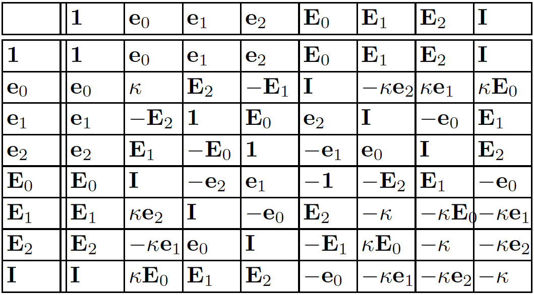
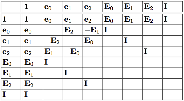
Multiplication table for 2D PGA. \(\kappa \in \{-1,0,1\}\)
1. We can normalize a proper line \(\mathbf{m}\) or point \(\mathbf{P}\) so that:$$\mathbf{m}^2 = 1,~~~\mathbf{P}^2 = -\kappa$$
1a. Elements such that \(\mathbf{x}^2=0\) are called ideal.
1b. Formulas given below often assume normalized arguments.
2. Multiplication with \(\mathbf{I}\): For any k-vector \(\mathbf{x}\), \(\mathbf{x}^\perp := \mathbf{x}\mathbf{I}\) is the orthogonal complement of \(\mathbf{x}\).
Example: \(\mathbf{e}_0 \mathbf{I} = \kappa\mathbf{e}_1\mathbf{e}_2\). The only thing left in \(\mathbf{I}\) is what isn't in \(\mathbf{X}\).
2a. In the euclidean case, \(\mathbf{I}^2=0\).
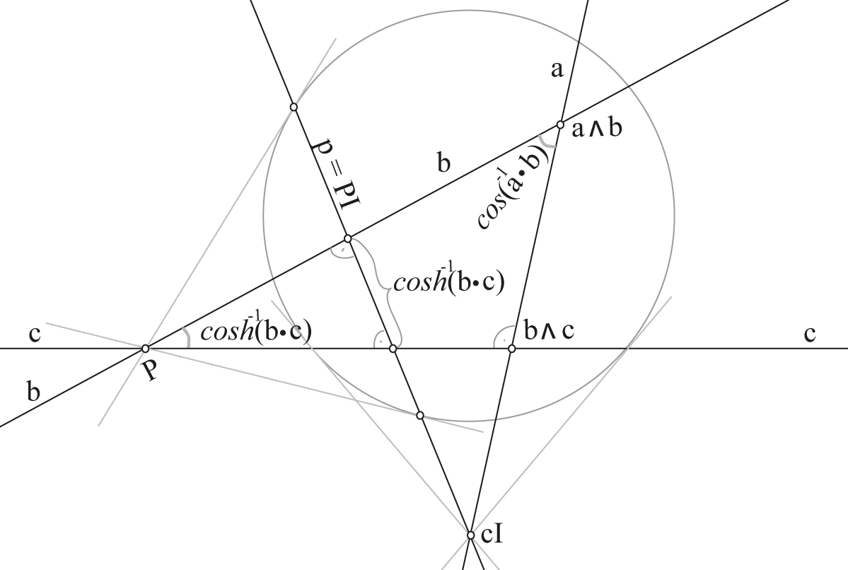
3. Product of two proper lines \(\mathbf{a},\mathbf{b}\) that meet at a proper point \(\mathbf{P}\):
$$\mathbf{a}\mathbf{b} = \cos(t) + \sin{(t)}\mathbf{P}$$
where \(t\) is the angle between the lines (arbitrary \(\kappa\)).
3a. Product of two proper lines \(\mathbf{a},\mathbf{b}\) \(\kappa = -1\), \(\mathbf{P}\) is hyper-ideal point. Then
$$\mathbf{a}\mathbf{b} = cosh(d) + \sinh(d)\mathbf{P}$$
where \(d\) is the hyperbolic distance between the lines.
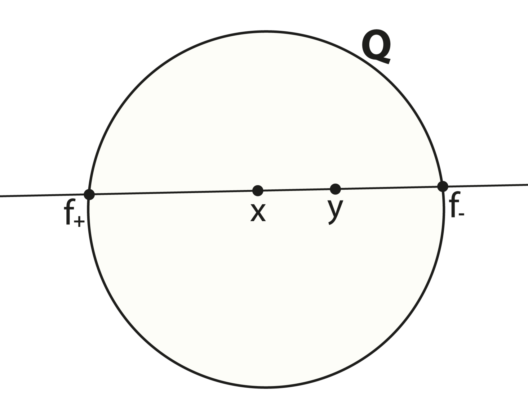
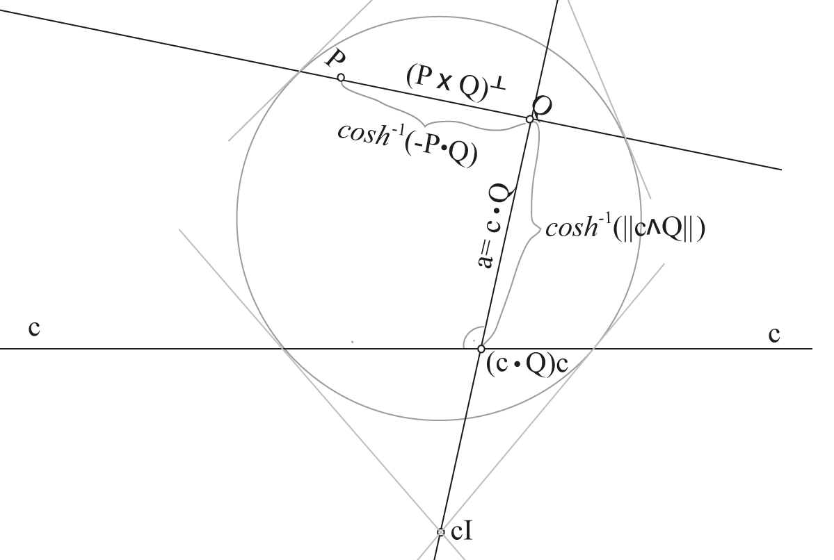
4. Product of proper line \(\mathbf{c}\) and proper point \(\mathbf{Q}\):
$$\mathbf{c}\mathbf{Q} = \mathbf{c} \cdot \mathbf{Q} + (\cosh{d)}\mathbf{I}~(=\langle cQ\rangle_1+\langle cQ \rangle_3)$$
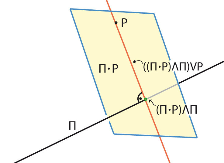
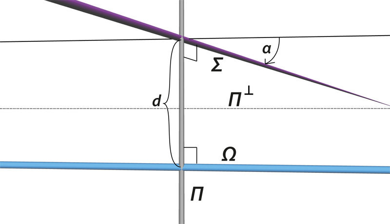
The first term is the line through \(\mathbf{Q}\) perpendicular to \(\mathbf{c}\), sometimes written \(\mathbf{a}^\perp_\mathbf{Q}\). \(d\) is the distance from point to line.
5. Product of two proper points \(\mathbf{P}, \mathbf{Q}\). Then
$$\mathbf{P}\mathbf{Q}=\cosh(d)+\sinh(d)\mathbf{R}$$
\(d\) is the distance between the two points and \(\mathbf{R}\) is the normalized form of \(\langle \mathbf{P}\mathbf{Q}\rangle_2\), which is the common orthogonal \((\mathbf{P}\vee\mathbf{Q})^\perp\).
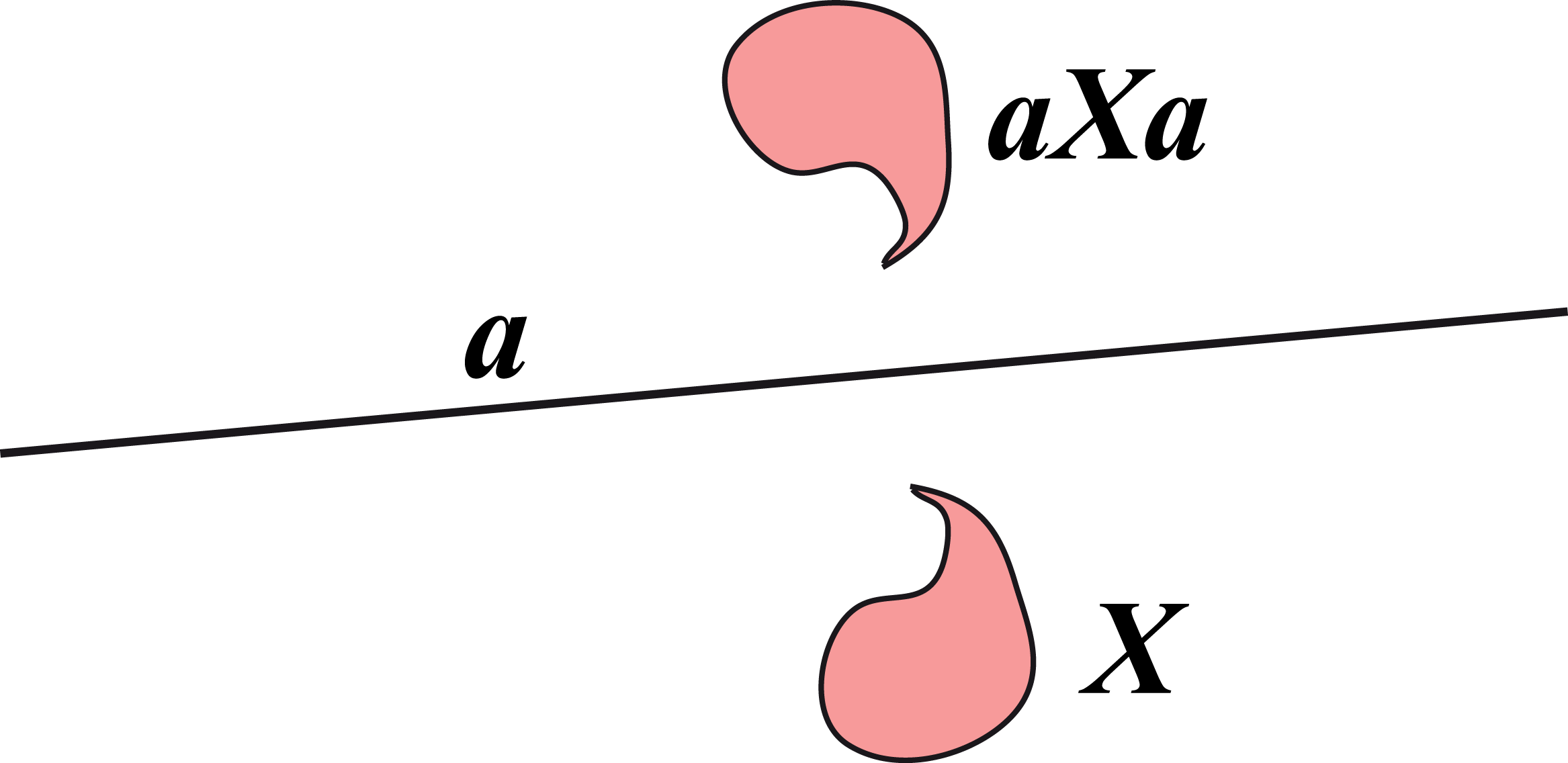
Reflections
Consider the 3-way product \(\mathbf{X}'=\mathbf{a}\mathbf{X}\mathbf{a}\), where \(\mathbf{a}\) is a proper line and \(\mathbf{X}\) is anything.
Then \(\mathbf{X}'\) is the reflection of \(\mathbf{X}\) in the line \(\mathbf{a}\).
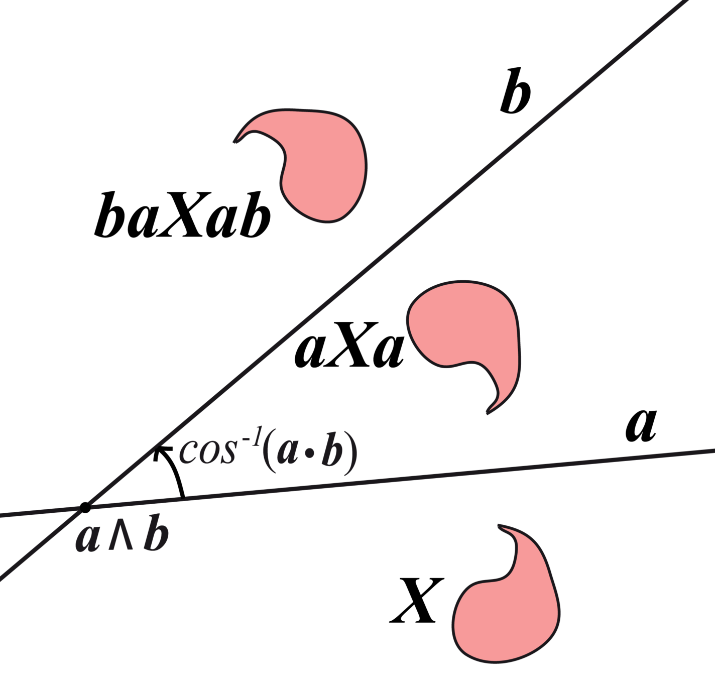
Rotations
A reflection in a second proper line \(\mathbf{b}\) gives \(\mathbf{X}'=\mathbf{b}(\mathbf{a}\mathbf{X}\mathbf{a})\mathbf{b} = (\mathbf{b}\mathbf{a})\mathbf{X}(\mathbf{a}\mathbf{b})\), by associativity. \(\mathbf{r}:=\mathbf{b}\mathbf{a}\) is called a rotor and \(X'=RX\widetilde{R}\) where \(\widetilde{R}\) is reversal operator.
Euclidean translations
If \(\kappa=0\) and \(\mathbf{P}\) is ideal, \(\mathbf{X}'\) is a translation of distance 2d, where d is the distance betwen a and b. Similar results for \(\kappa = -1\).
For \(\kappa=1\), the even sub-algebra (shown in red) is isomorphic to \(\mathbb{H}\) under the map $$\{1,\mathbf{E}_0,\mathbf{E}_1,\mathbf{E}_2\}\Leftrightarrow\{1,\mathbf{k},\mathbf{j},\mathbf{i}\}$$
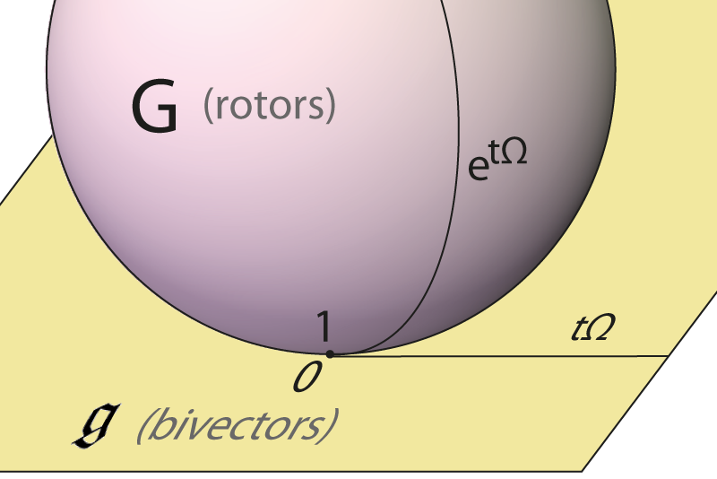
Every rotor can be produced directly by exponentation of a bivector. When \(\mathbf{P}^2=-1\) then
$$\mathbf{r} := \exp(t\mathbf{P}) = \cos(t) + \sin(t)\mathbf{P}$$
\(\mathbf{r}\mathbf{X}\widetilde{\mathbf{r}}\) produces a rotation through angle \(2t\) around \(\mathbf{P}\).
Analogous results hold for \(\mathbf{P}^2=0 \text{ or } 1\) yielding parabolic or hyperbolic isometries.
The ideal norm
\(\mathbf{P}^2 = 0\): how to normalize \(\mathbf{P}\) so \(e^{dP}\) is a translation of 2d? Time permitting ...
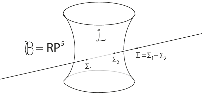
The bivectors \(\bigwedge^2\) form the Lie algebra.
Define \(\mathbf{G}\) to be the elements of the even sub-algebra of norm 1. Then \(\mathbf{G}\) is the Lie group.
And \(\exp: \bigwedge^2 \rightarrow \mathbf{G}\) is a 1:1 map up to multiples of \(2\pi\) (for \(n=3\)).
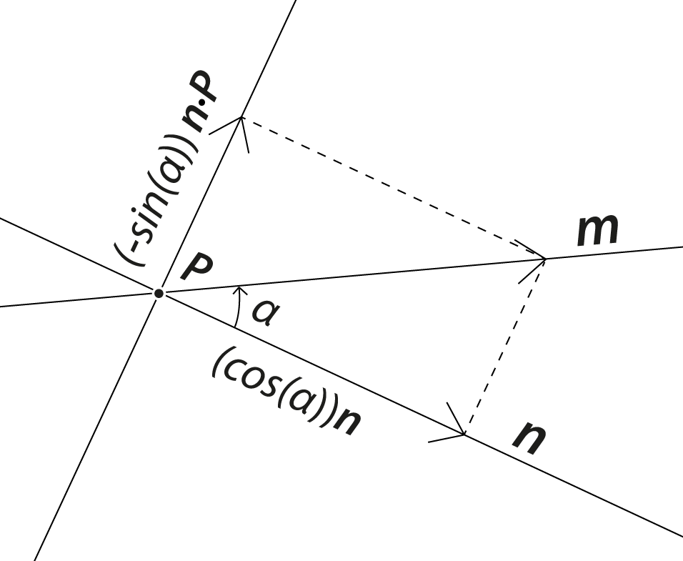
3-way products with a repeated factor of the form \(\mathbf{Y}\mathbf{X}\mathbf{X}\) can be used as formula factories.
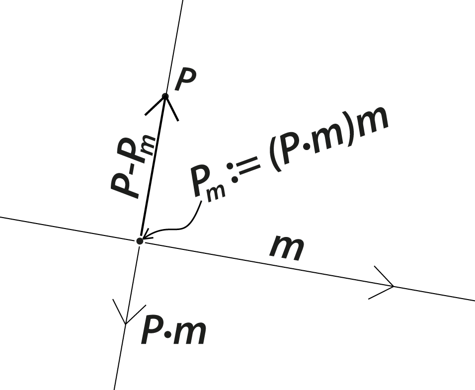
Example: \(\mathbf{m} = \mathbf{m}(\mathbf{n}\mathbf{n}) = (\mathbf{m}\mathbf{n})\mathbf{n} \) since for a proper line \(\mathbf{n}^2 = 1\) and associativity. This leads to a decomposition of \(\mathbf{m}\) with respect to \(\mathbf{n}\):
$$(mn)n=(\cos(\alpha)+\sin(\alpha)\mathbf{P})n$$
$$=\cos(\alpha)n + \sin(\alpha)Pn$$
$$=\cos(\alpha)n +\sin(\alpha)P\cdot n$$
$$=\cos(\alpha)n - \sin(\alpha)n\cdot P$$
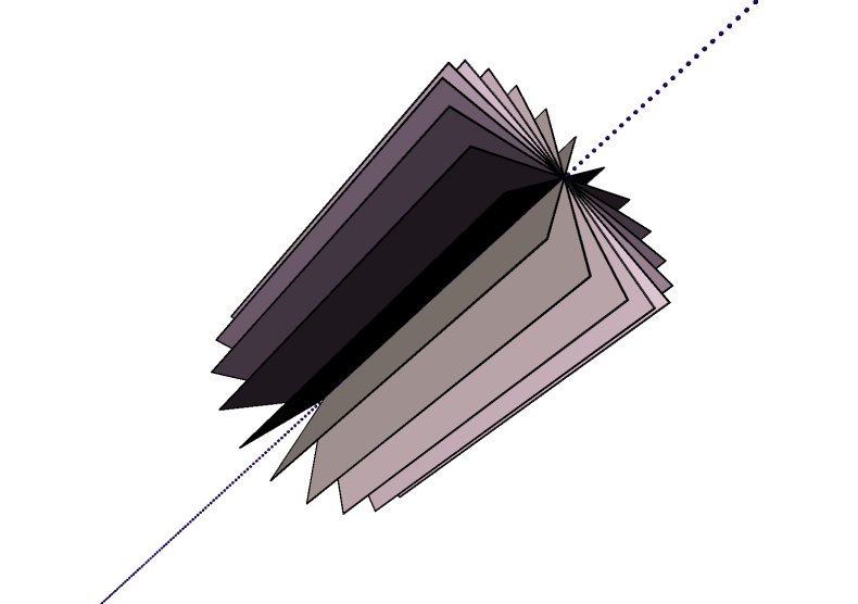
The arrows show the orientation of the lines.
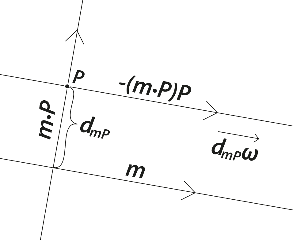
Examples: Anything can be orthogonally decomposed with respect to anything else! For example ...
Decompose point WRT line.
Decompose line WRT point.
The pieces of the decomposition are often interesting in their own right. For example, \((P\cdot m)m\) is closest point to \(P\) on \(m\).
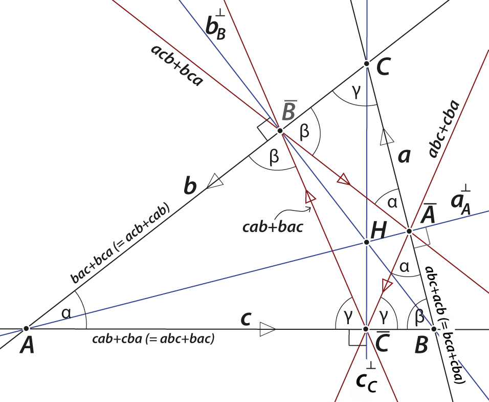
General 3-way products \(\mathbf{a}\mathbf{b}\mathbf{c}\) of 1-vectors provide a useful framework for a general theory of triangles. Lots left to do!
A euclidean demo from Steven De Keninck, using his ganja.js Javascript implementation, showing several of the features discussed above.
\(\ell\) = line (vector)
\(P\) = point (bivector)
\(\ell P\) = line through \(P, \perp\) to \(\ell\)
\(\ell P\ell\) = reflection of \(P\) in \(\ell\)
\(P\ell P\) = reflection of \(\ell\) in \(P\)
\((\ell \cdot P)\ell\) = projection of \(P\) on \(\ell\)
\((P \cdot \ell)P\) = projection of \(\ell\) on \(P\)
Live slides are available at https://slides.com/charlieboy/icerm2019/
Bivectors!
Julius Pluecker
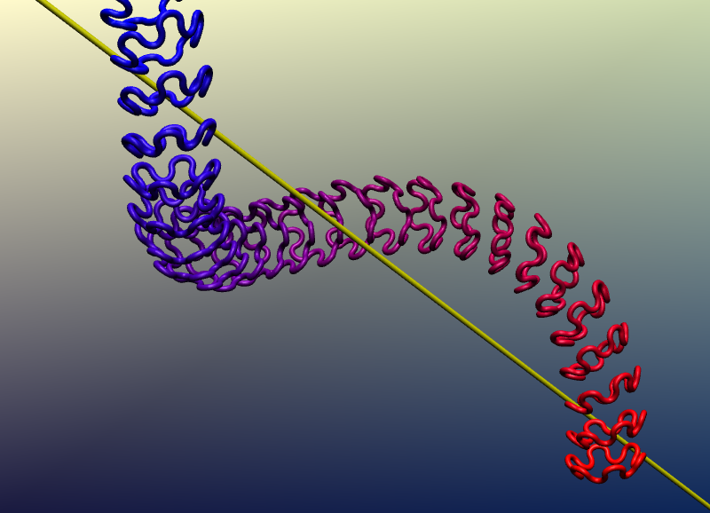
A velocity state is \( \mathbf{V} \in \bigwedge^2\) (in this case a point)
A momentum state is \(\mathbf{M} \in \bigwedge^{n-2}\) (in this case a line)
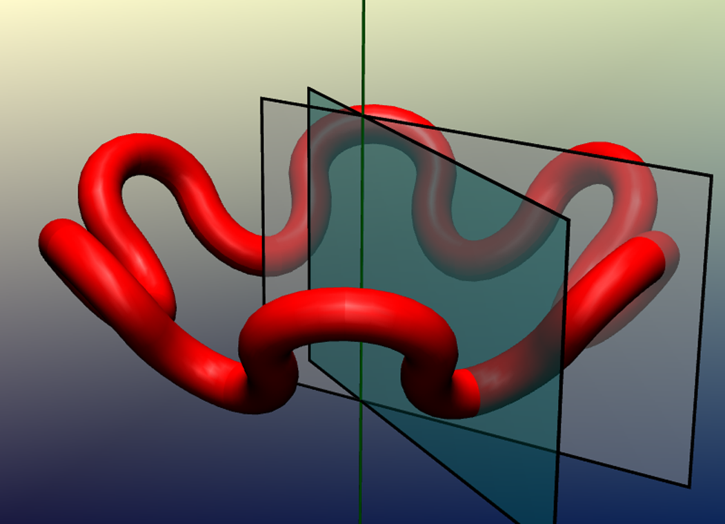
A rigid body is a collection of Newtonian mass points.
Calculate inertia tensor \(A\) for the body, a quadratic form determined by the mass distribution.
\(\mathbf{M}=A\mathbf{V}\)
ODE's for free top:
PGA equations for the free top in \(P(\mathbb{R}^*_{\kappa})\):
$$\dot{\mathbf{g}} = \mathbf{g} \mathbf{V}~~~~~~~~$$ $$~~~~~~~~~~~ \dot{\mathbf{M}} = \frac12(\mathbf{V}\mathbf{M} - \mathbf{M} \mathbf{V}) $$
where \(\mathbf{g} \in \mathbf{G}\), and \(\mathbf{M}\) and \( \mathbf{V} \)are in the body frame.
Advantages of PGA:
3D
Poinsot motion (?)
Coordinate-free
Uniform rep'n for points, lines, and planes
Single, uniform rep'n for isometries
Parallel-safe meet and join operators
Compact expressions for classical geometric results
Physics-ready
Metric-neutral
Backwards compatible
Metric-neutral resources
Euclidean resources
Questions and comments: projgeom at gmail.com
Thanks for your attention!
That's all folks
Quaternions \(\mathbb{H}\)
Im. quaternions \(\mathbb{IH}\)
Unit quaternions \(\mathbb{U} \)
$$s+x\mathbf{i}+y\mathbf{j}+z\mathbf{k}$$
$$ \mathbf{v} := x\mathbf{i}+y\mathbf{j}+z\mathbf{k} \Leftrightarrow (x,y,z) \in \mathbb{R}^3 $$
$$\{\mathbf{g}\in\mathbb{H} \mid \mathbf{g}\overline{\mathbf{g}}= 1\}$$
III. ODE's for Euler top:
Quaternion equations for the Euler top in \(\mathbb{R}^3\):
$$\dot{\mathbf{g}} = \mathbf{g} \mathbf{V}$$ $$ \dot{\mathbf{M}} = \frac12(\mathbf{V}\mathbf{M} - \mathbf{M} \mathbf{V}) $$
where \(\mathbf{g} \in \mathbb{U}\) and \(\mathbf{M}, \mathbf{V} \in \mathbb{IH}\) are the momentum, resp., velocity vectors in the body frame.
(\(\mathbf{M}={A}\mathbf{V}\) for inertia tensor \(A\)).
Multiplication table for \(\bigwedge\mathbb{R}P^{2\large{*}}\)
Question: Why is the signature \((2,0,1)\) using the dual construction the proper model for the euclidean plane?
Answer: Given two lines \(\mathbf{m}_i = c_i\mathbf{e}_0+a_i\mathbf{e}_1+b_i\mathbf{e}_2\) (with equations \(a_ix+b_iy+c_i=0\)). Then $$\mathbf{m}_1\cdot\mathbf{m}_2=c_0c_1\mathbf{e}_0^2+a_1a_2\mathbf{e}_1^2+b_1b_2\mathbf{e}_2^2$$ Since the cosine of the angle between the lines is \(a_1a_2 + b_1b_2\), \(\mathbf{e}_0^2=0\) while \(\mathbf{e}_1^2=\mathbf{e}_2^2=1\).
History: That \(\mathbf{P}(\mathbb{R}^*_{2,0,1}) \) models euclidean geometry was first published by Jon Selig in 2000.
By Charles Gunn
Geometric algebra for Cayley-Klein spaces: a Swiss army knife for graphics and games


