ORIGIN - Bloch

Bloch function: periodic function modulated by plane waves.

\displaystyle \psi_{n \mathbf{k}}(\mathbf{r})=u_{n \mathbf{k}}(\mathbf{r}) e^{i \mathbf{k} \cdot \mathbf{r}}

\displaystyle \psi_{n \mathbf{k}}(\mathbf{r})=u_{n \mathbf{k}}(\mathbf{r}) e^{i \mathbf{k} \cdot \mathbf{r}}

k vectors come from cell periodicity. i.e. for 1D:

\displaystyle \mathbf{k} = \frac{2\pi}{N\cdot \mathbf{a}} n; n \in (0,1,2,3, \cdots)

\displaystyle \mathbf{k} = \frac{2\pi}{N\cdot \mathbf{a}} n; n \in (0,1,2,3, \cdots)

\displaystyle =

\displaystyle =

\displaystyle \times

\displaystyle \times

ORIGIN - reverse?

By doing DFT, we are using basis functions to describe Bloch functions:

Can reverse this process?

Basis (PW, local set)

DFT calculator

Bloch WFs

???

Basis (PW, local set)

This question is particularly interesting because if we have a DFT WF calculated with PW basis, reverting to a minimum atomic basis will give us much chemical intuition + speed if we want to do other stuff with them.

ORIGIN - FT

We can use these envelope function to construct localized functions with Fourier transform (AKA superposition of Bloch functions 🤪)

\displaystyle \begin{aligned} \mathscr{F}_{\mathbf{k}} \{ \psi_{n \mathbf{k}}(\mathbf{r}) \} (\mathbf{R}) &\sim \int_{-\infty}^{\infty} u_{n \mathbf{k}}(\mathbf{r}) e^{i \mathbf{k} \cdot \mathbf{r}} e^{i \mathbf{k} \cdot \mathbf{R}} \mathrm{d} \mathbf{k} \\ &= u_{n \mathbf{k}}(\mathbf{r}) \delta(\mathbf{r}-\mathbf{R}) = u_{n \mathbf{k}}(\mathbf{R}) \end{aligned}

\displaystyle \begin{aligned} \mathscr{F}_{\mathbf{k}} \{ \psi_{n \mathbf{k}}(\mathbf{r}) \} (\mathbf{R}) &\sim \int_{-\infty}^{\infty} u_{n \mathbf{k}}(\mathbf{r}) e^{i \mathbf{k} \cdot \mathbf{r}} e^{i \mathbf{k} \cdot \mathbf{R}} \mathrm{d} \mathbf{k} \\ &= u_{n \mathbf{k}}(\mathbf{r}) \delta(\mathbf{r}-\mathbf{R}) = u_{n \mathbf{k}}(\mathbf{R}) \end{aligned}

However, we don't have infinite k points, we only have k-points live inside the BZ, this means our delta function is not a delta function, but a modulation with finite width that's localized on the R lattice!

\rightarrow

\rightarrow

Definition

The formal definition of a Wannier function from a single Bloch band:

Wannier transformation

\displaystyle w_{\mathbf{R}}(\mathbf{r})=\frac{V}{(2 \pi)^{3}} \int_{\mathrm{BZ}} \psi_{\mathbf{k}}(\mathbf{r}) e^{-\mathrm{ik} \cdot \mathbf{R}} \mathrm{d} \mathbf{k}

\displaystyle w_{\mathbf{R}}(\mathbf{r})=\frac{V}{(2 \pi)^{3}} \int_{\mathrm{BZ}} \psi_{\mathbf{k}}(\mathbf{r}) e^{-\mathrm{ik} \cdot \mathbf{R}} \mathrm{d} \mathbf{k}

Gauge freedom

However, Bloch functions have another degree of freedom: gauge freedom:

\displaystyle |\tilde{\psi}_{n \mathbf{k}}\rangle=e^{i \varphi_{n}(\mathbf{k})}\left|\psi_{n \mathbf{k}}\right\rangle

\displaystyle |\tilde{\psi}_{n \mathbf{k}}\rangle=e^{i \varphi_{n}(\mathbf{k})}\left|\psi_{n \mathbf{k}}\right\rangle

This transformation changes nothing about the physical description of the system.
However, the "smoothness" of our Wannier function depends on the smoothness of the Bloch function in k space.

Multiband

For multi-band situation, we can construct another set of bloch functions:

\displaystyle |\tilde{\psi}_{n \mathbf{k}} \rangle=\sum_{m=1}^{J} U_{m n}^{(\mathbf{k})}\left|\psi_{m \mathbf{k}}\right\rangle

\displaystyle |\tilde{\psi}_{n \mathbf{k}} \rangle=\sum_{m=1}^{J} U_{m n}^{(\mathbf{k})}\left|\psi_{m \mathbf{k}}\right\rangle

U is an unitary matrix so this is a unitary rotation, which means:
- the charge density is not changed
- $|\tilde{\psi}_{n \mathbf{k}} \rangle$ still form a orthonormal set.

Definition +

For multi-band situation, the Wannier transformation:

\displaystyle w_{n \mathbf{R}}(\mathbf{r})=\frac{V}{(2 \pi)^{3}} \int_{\mathrm{BZ}}\left[\sum_{m} U_{m n}^{(\mathbf{k})} \psi_{m \mathbf{k}}(\mathbf{r})\right] e^{-\mathrm{i} \mathbf{k} \cdot \mathbf{R}} \mathrm{d} \mathbf{k}

\displaystyle w_{n \mathbf{R}}(\mathbf{r})=\frac{V}{(2 \pi)^{3}} \int_{\mathrm{BZ}}\left[\sum_{m} U_{m n}^{(\mathbf{k})} \psi_{m \mathbf{k}}(\mathbf{r})\right] e^{-\mathrm{i} \mathbf{k} \cdot \mathbf{R}} \mathrm{d} \mathbf{k}

The inverse transformation:

\displaystyle \psi_{m \mathbf{k}}(\mathbf{r}) = \sum_{\mathbf{R}} e^{i\mathbf{k}\mathbf{R}} w_{n \mathbf{R}}(\mathbf{r})

\displaystyle \psi_{m \mathbf{k}}(\mathbf{r}) = \sum_{\mathbf{R}} e^{i\mathbf{k}\mathbf{R}} w_{n \mathbf{R}}(\mathbf{r})

Projection

In order to get an initial unitary matrix, we project the Bloch functions onto a set of localized functions $|g_n\rangle$ :

\displaystyle \left|\phi_{n \mathbf{k}}\right\rangle=\sum_{m=1}^{J}\left|\psi_{m \mathbf{k}}\right\rangle\left\langle\psi_{m \mathbf{k}}|g_{n}\right\rangle

\displaystyle \left|\phi_{n \mathbf{k}}\right\rangle=\sum_{m=1}^{J}\left|\psi_{m \mathbf{k}}\right\rangle\left\langle\psi_{m \mathbf{k}}|g_{n}\right\rangle

But $\left|\phi_{n \mathbf{k}}\right\rangle$ does not form a orthornomal set, we need to orthonormalize them by using overlap matrix $S_\mathbf{k}=\langle\phi_{n\mathbf{k}}|\phi_{n\mathbf{k}}\rangle$ :

\displaystyle |\tilde{\psi}_{n \mathbf{k}}\rangle=\sum_{m=1}^{J}\left|\phi_{m \mathbf{k}}\right\rangle\left(S_{\mathbf{k}}^{-1 / 2}\right)_{m n}

\displaystyle |\tilde{\psi}_{n \mathbf{k}}\rangle=\sum_{m=1}^{J}\left|\phi_{m \mathbf{k}}\right\rangle\left(S_{\mathbf{k}}^{-1 / 2}\right)_{m n}

Entanglement

Normally we don't need this but if we have the following case (graphene, $p_z$ on C):

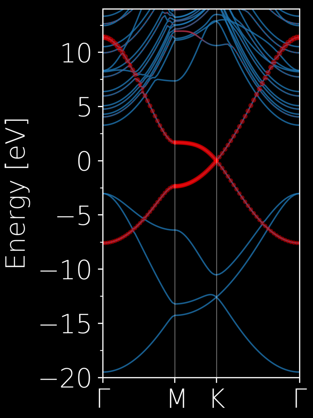
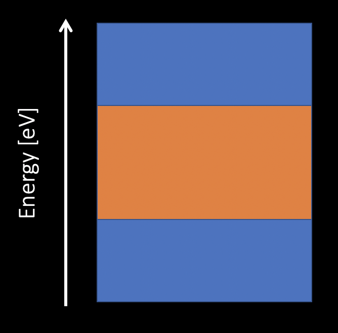
No entanglement

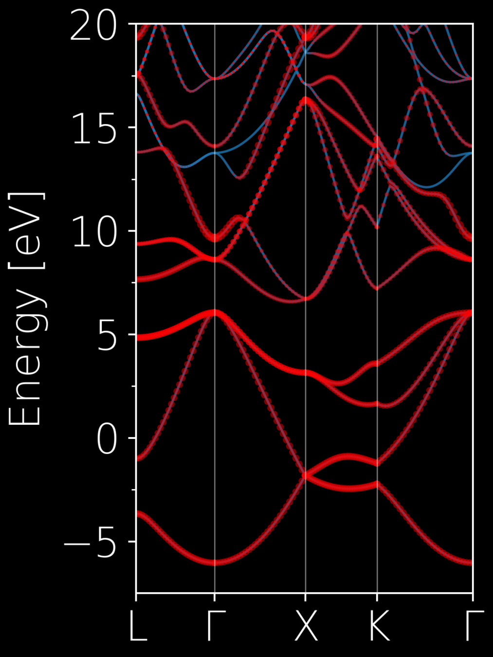
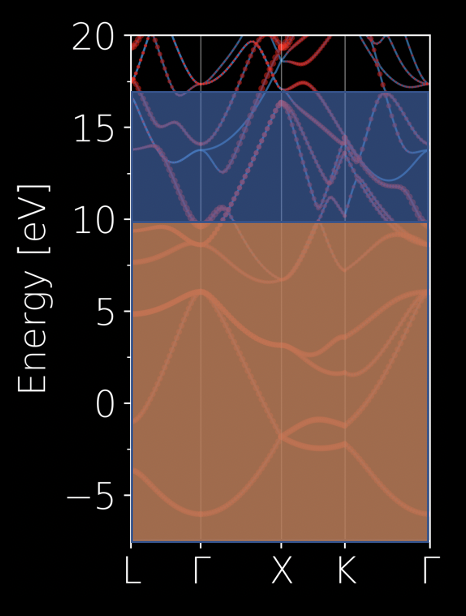
Entanglement

We can use another $U_{mn}^{\mathrm{(pre)}}$ to do the band selection!

SPread function

Even tough now we have a unary matrix, Wannier functions are still non-unique and depend on the original projectors used.
Introducing - spread function:

\displaystyle \Omega=\sum_{n}\left[\left\langle\mathbf{0} n\left|r^{2}\right| \mathbf{0} n\right\rangle-\langle\mathbf{0} n|\mathbf{r}| \mathbf{0} n\rangle^{2}\right]=\sum_{n}\left[\left\langle r^{2}\right\rangle_{n}-\overline{\mathbf{r}}_{n}^{2}\right]

\displaystyle \Omega=\sum_{n}\left[\left\langle\mathbf{0} n\left|r^{2}\right| \mathbf{0} n\right\rangle-\langle\mathbf{0} n|\mathbf{r}| \mathbf{0} n\rangle^{2}\right]=\sum_{n}\left[\left\langle r^{2}\right\rangle_{n}-\overline{\mathbf{r}}_{n}^{2}\right]

Essentially, this is a squared deviation from mean in real space. We can keep on changing the unitary matrix to minimize this function.
To calculate this we need (details not shown):

\displaystyle M_{m n}^{(\mathbf{k}, \mathbf{b})}=\left\langle u_{m \mathbf{k}} \mid u_{n, \mathbf{k}+\mathbf{b}}\right\rangle

\displaystyle M_{m n}^{(\mathbf{k}, \mathbf{b})}=\left\langle u_{m \mathbf{k}} \mid u_{n, \mathbf{k}+\mathbf{b}}\right\rangle

Maximally localized Wannier function!

Procedure -VASP

Run a single point calculation, write charge density and wave functions files.
"Fat band" calculation to determine the energy window and bands to Wannierize.
Write a wannier90.win file.
Continue previous DFT calculation with:
- ALGO = None
- LWANNIER90 = .T.
Run wannier90.x to get unitary matrices.
Do whatever post processing you want 🪄.

Things needeD

From DFT calculations:
- .amn file: projection coefficients
- .mmn file: overlap coefficients
- UNK.* files (optional): periodic part of the Bloch functions for plotting purpose.
From input (wannier90.win file):
- number of target Wannier functions
- DFT bands: how many, what to exclude
- initial projection (guiding) functions

A typical .WIN file

# band indeices starts from 0
num_bands         =   7
num_wann          =   4
exclude_bands     =   8-16

# total window
dis_win_max       =  20.0
dis_win_min       =  -7.5

# frozen window
dis_froz_max      =  6.2
dis_froz_min      =  -7.5

# disentanglement control
#dis_num_iter      =  120
#dis_mix_ratio     =  1.d0
num_iter          =  0
num_print_cycles  =  10

# projection section
Begin Projections
c=0.0,0.0,0.0:sp3
End Projections

Lets calculate!

Energy Windows

There are 4 tags to control the energy windows:

dis_win_max

dis_win_min

dis_froz_max

dis_froz_min

blue region: disentanglement
Orange region: no disentanglement

Energy Windows

Use fat band analysis determine the windows.

For this example, by projecting on to s and p orbitals of silicon, we need a total of 8 bands (two atoms, each with 4 orbitals).

Energy Windows

So, we need dis_win_max and dis_win_min to contain more than 8 bands.
dis_froz_max and dis_froz_min should contain less than 8 bands and the bands inside this range should have more apparent contribution from s and p orbitals from Si atoms.

Energy Windows

dis_win_max: 17 eV

dis_win_min: -7.5 eV

dis_froz_max: 10 eV

dis_froz_min: -7.5 eV

Projection only

Often times running spread minimization procedure causes the lost of symmetry in Wannier functions or other undesired behaviors.

To avoid this, we can run "projection-only" Wannierzation by setting the following in wannier90.win:
- num_iter = 0

Plotting WF

To plot Wannier function, put the following to your INCAR along side LWANNIER90=.T. when generating Wannier inputs:
- LWRITE_UNK=.T.
And in wannier90.win file, add something like :
- wannier_plot = true
- wannier_plot_list = 1 2 3
- wannier_plot_supercell = 5 5 1
the Im/Re ratio for each of the Wannier functions are written in the wannier90.wout file.

Quanlity control

What attributes can we determine if we have a good Wannier functions or not?
- Real function: check Im/Re ratio of the WFs.
- Minimum spread: check spread < cell.
- Can reproduce DFT band structure.
- Generally, matches your chemical intuition. 👻

Tips & Tricks

If a projection only calculation is viable, do that!
Play with projection (guiding) functions, try changing their orientation and shape (see manual, chapter 3).
Place s orbital on bond center and run minimization procedure.
use guiding_centres=.T. in wannier90.win

Resouces

Wannier90's Manual & Tutorials 😹
Nicola Marzari, et al, Rev. Mod. Phys. 84, 1419, 2012

Some names to remember:
- G. H. Wannier: inventor of Wannier function
- N. Marzari and D. Vanderbilt: localization criteria
- I. Souza: disentanglement

Other stuff

VASP2Wannier90 interface: duh
WanOCC: Wannier occupation matrix
WanSOC: Add SOC to Wannier Hamiltonian
WanPB: Interface to Pybinding
WOBSTER: Wannier orbital overlap population
WOOPs: WOBSTER but in real space.

☄️Some of my work that has something to do with Wannier90:

ORIGIN - Bloch

ORIGIN - reverse?

ORIGIN - FT

Definition

Gauge freedom

Multiband

Definition +

Projection

Entanglement

SPread function

What DO we need?

Procedure -VASP

Things needeD

A typical .WIN file

Lets calculate!

Energy Windows

Energy Windows

Energy Windows

Energy Windows

Projection only

Plotting WF

Quanlity control

Tips & Tricks

Resouces

Other stuff

thank you 🤟

Questions?

2021-11-06-W90 short tutorial

2021-11-06-W90 short tutorial

Chengcheng Xiao

ORIGIN - Bloch

ORIGIN - reverse?

ORIGIN - FT

Definition

Gauge freedom

Multiband

Definition +

Projection

Entanglement

SPread function

What DO we need?

Procedure -VASP

Things needeD

A typical .WIN file

Lets calculate!

Energy Windows

Energy Windows

Energy Windows

Energy Windows

Projection only

Plotting WF

Quanlity control

Tips & Tricks

Resouces

Other stuff

thank you 🤟

Questions?

2021-11-06-W90 short tutorial

More from Chengcheng Xiao