


Kevin Song
I'm a student at UT (that's the one in Austin) who studies things.
A family of computational techniques to find key points in time series data where the behavior of the data changes (hence the name "changepoint").
Assumes that time-series data is drawn piecewise from stationary distributions.
Time
For convenience we'll also assume data are read at a consistent dt. (Not strictly needed, but math becomes a lot cleaner).
Time
Assumes that time-series data is drawn piecewise from stationary distributions.
Assumes that time-series data is drawn piecewise from stationary distributions.
Time
Time
Assumes that time-series data is drawn piecewise from stationary distributions.
Time
Assumes that time-series data is drawn piecewise from stationary distributions.
Time
Assumes that time-series data is drawn piecewise from stationary distributions.
Time
Assumes that time-series data is drawn piecewise from stationary distributions.
Time
At certain key times \( \{t_i^*\} \), we switch between different distributions.
Assumes that time-series data is drawn piecewise from stationary distributions.
Time
At certain key times \( \{t_i^*\} \), we switch between different distributions.
Assumes that time-series data is drawn piecewise from stationary distributions.
Time
At certain key times \( \{t_i^*\} \), we switch between different distributions.
Assumes that time-series data is drawn piecewise from stationary distributions.
Time
At certain key times \( \{t_i^*\} \), we switch between different distributions.
Assumes that time-series data is drawn piecewise from stationary distributions.
Time
At certain key times \( \{t_i^*\} \), we switch between different distributions.
Assumes that time-series data is drawn piecewise from stationary distributions.
Time
At certain key times \( \{t_i^*\} \), we switch between different distributions.
Assumes that time-series data is drawn piecewise from stationary distributions.
Time
At certain key times \( \{t_i^*\} \), we switch between different distributions.
Assumes that time-series data is drawn piecewise from stationary distributions.
Time
At certain key times \( \{t_i^*\} \), we switch between different distributions.
Assumes that time-series data is drawn piecewise from stationary distributions.
Time
Of course, we don't get to see what the distributions are or which distribution the points come from!
Time
Of course, we don't get to see what the distributions are or which distribution the points come from!
Time
C. Truong, L. Oudre, N. Vayatis. Selective review of offline change point detection methods. Signal Processing, 167:107299, 2020.
This implicitly assumes a Gaussian with fixed variance and unknown mean (it is the MLE likelihood for the estimator of such a distribution under the given data). Other likelihoods assume unknown mean/variance, Poisson distributions, etc.
To find the overall cost of some proposed segmentation \( \{t_i\} \), we compute:
Penalty term to prevent too many changepoints.
Time
Time
Time
Time
Time
Time
Time
Time
Time
Time
Time
Use search algorithms (e.g. greedy binary segementation, dynamic programming, PELT) to find a "good" set of changepoints. Global optimality is often unfeasible.
A work in progress.....
Bayesian Information Criterion has proven helpful to get a starting point, but tends to underestimate the number of changepoints in the true data.
Possible to target known mean transition rate in data.
| HMM | Changepoint | |
|---|---|---|
| Inputs |
Time
| HMM | Changepoint | |
|---|---|---|
| Inputs |
Time
| HMM | Changepoint | |
|---|---|---|
| Inputs |
Time
| HMM | Changepoint | |
|---|---|---|
| Inputs | Photon data, kinetic scheme, and an emission model (latter two usually unknown parameters + initial guesses) | Data and an emission model |
Time
| HMM | Changepoint | |
|---|---|---|
| Inputs | Photon data, kinetic scheme, and an emission model (latter two usually unknown parameters + initial guesses) | Data and an emission model |
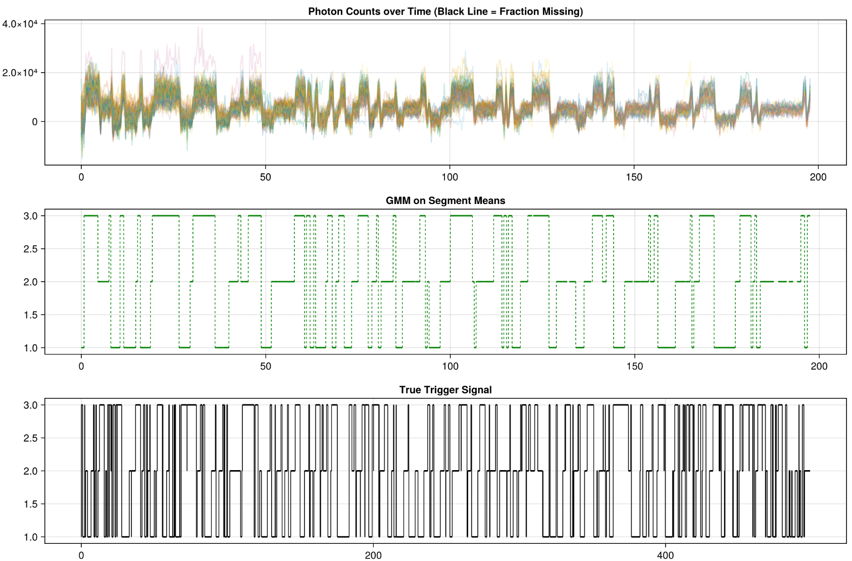
| Outputs (Phase 1) |
1.0
3.0
5.0
Time
| HMM | Changepoint | |
|---|---|---|
| Inputs | Photon data, kinetic scheme, and an emission model (latter two usually unknown parameters + initial guesses) | Data and an emission model |
| Outputs (Phase 1) | Kinetic Rates | Changepoints |
1.0
3.0
5.0
Time
1.0
3.0
5.0
Time
| HMM | Changepoint | |
|---|---|---|
| Inputs | Photon data, kinetic scheme, and an emission model (latter two usually unknown parameters + initial guesses) | Data and an emission model |
| Outputs (Phase 1) | Kinetic Rates | Changepoints |
| Outputs (Phase 2) |
1.0
3.0
5.0
Time
| HMM | Changepoint | |
|---|---|---|
| Inputs | Photon data, kinetic scheme, and an emission model | Data and an emission model |
| Outputs (Phase 1) | Kinetic Rates | Changepoints |
| Outputs (Phase 2) | Assignment of changepoints to states |
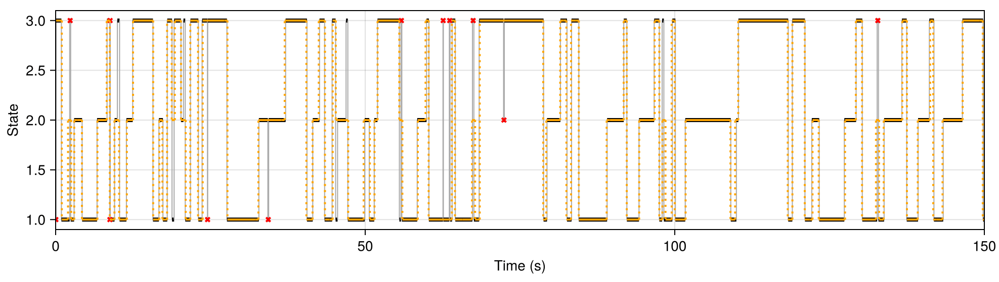
Synthetic process:
= Triggering Trajectory
= Recovered Trajectory
= States shorter than 0.25s
x
= Triggering Trajectory
= Recovered Trajectory
= States shorter than 0.25s
x
= Triggering Trajectory
= Recovered Trajectory
= States shorter than 0.25s
x
= Triggering Trajectory
= Recovered Trajectory
= States shorter than 0.25s
x
= Triggering Trajectory
= Recovered Trajectory
= States shorter than 0.25s
x
= Triggering Trajectory
= Recovered Trajectory
= States shorter than 0.25s
x
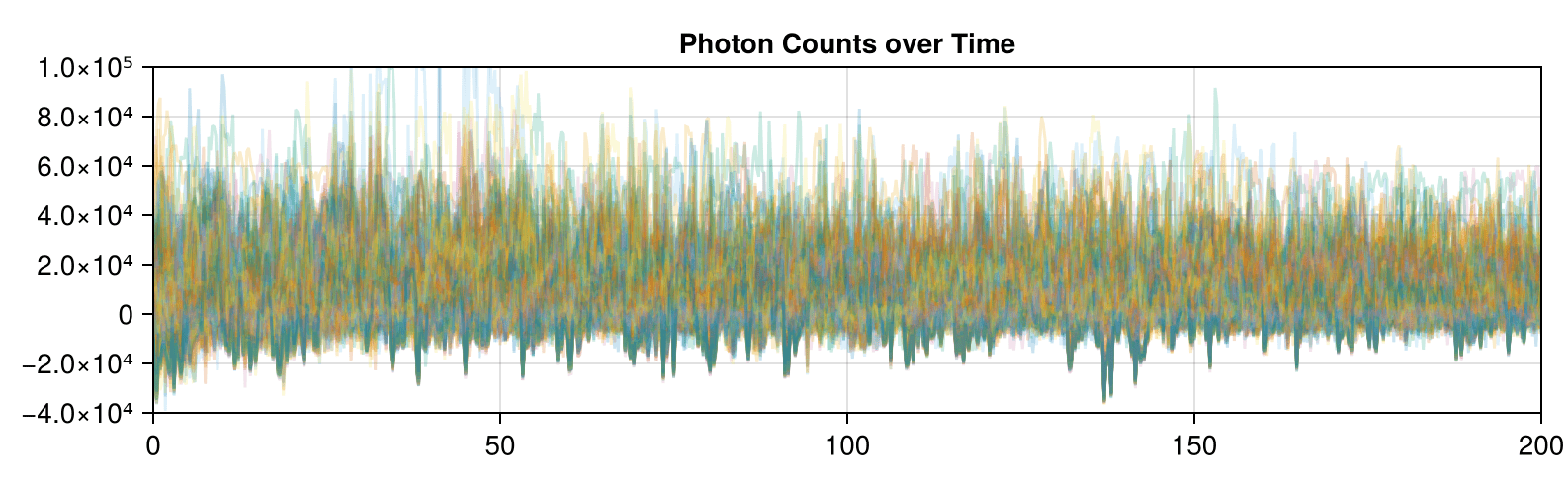
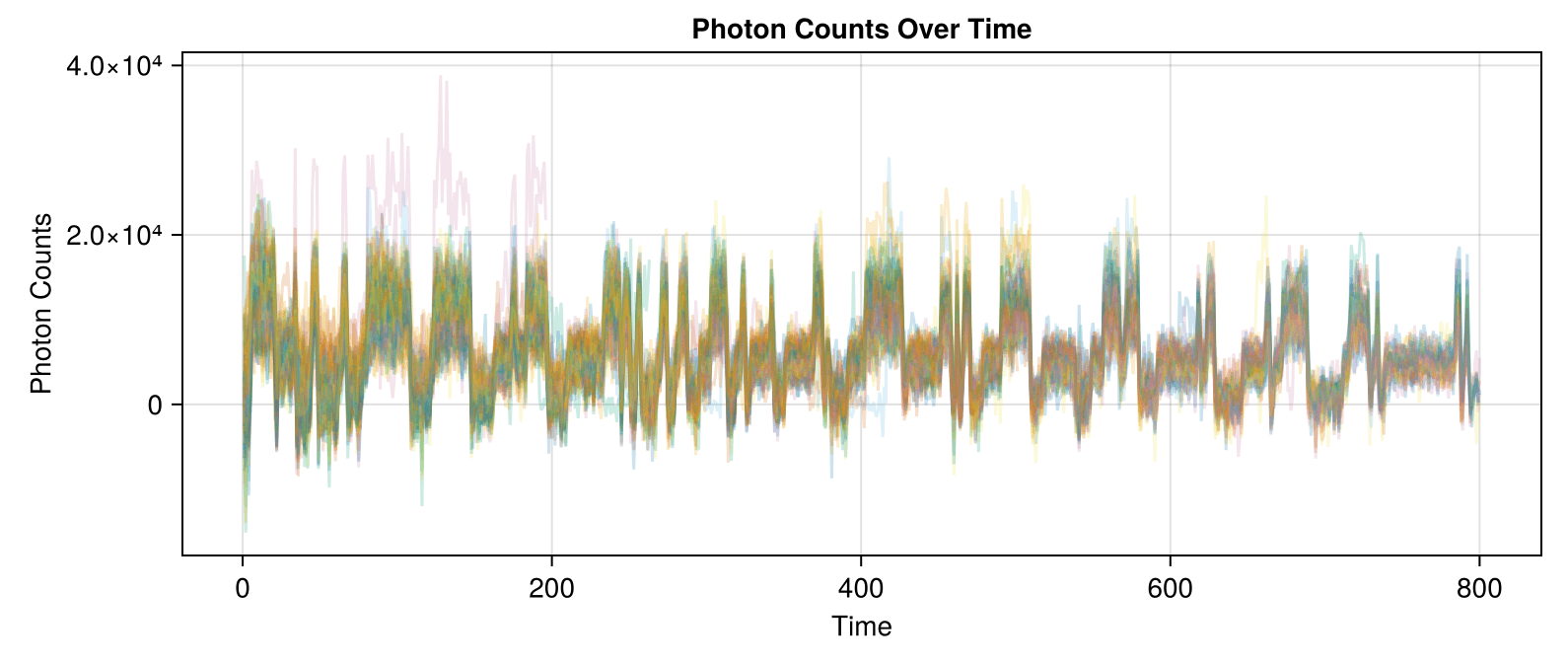
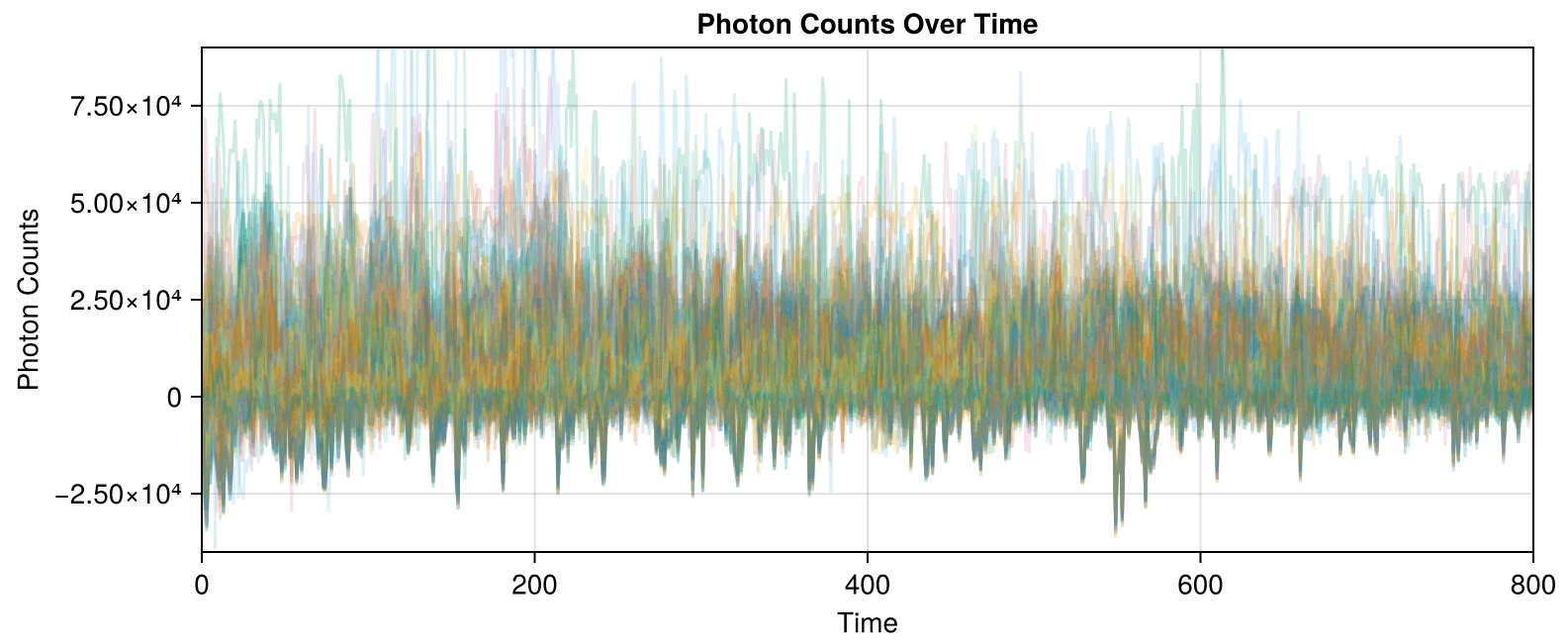
But if we eyeball the photon data, the missing transitions seem totally unrecoverable.
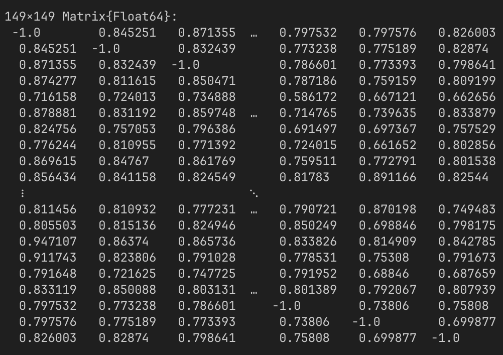
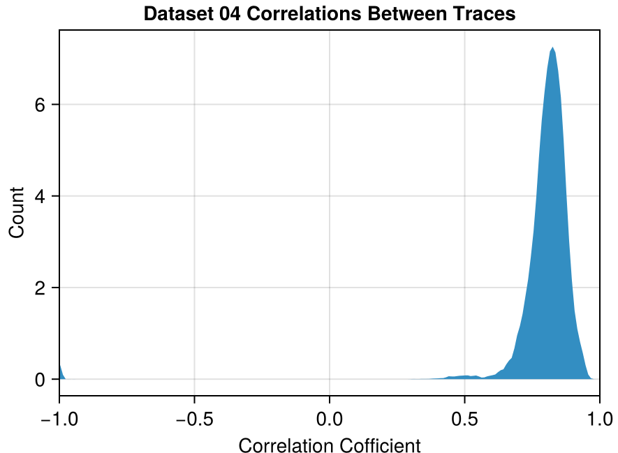
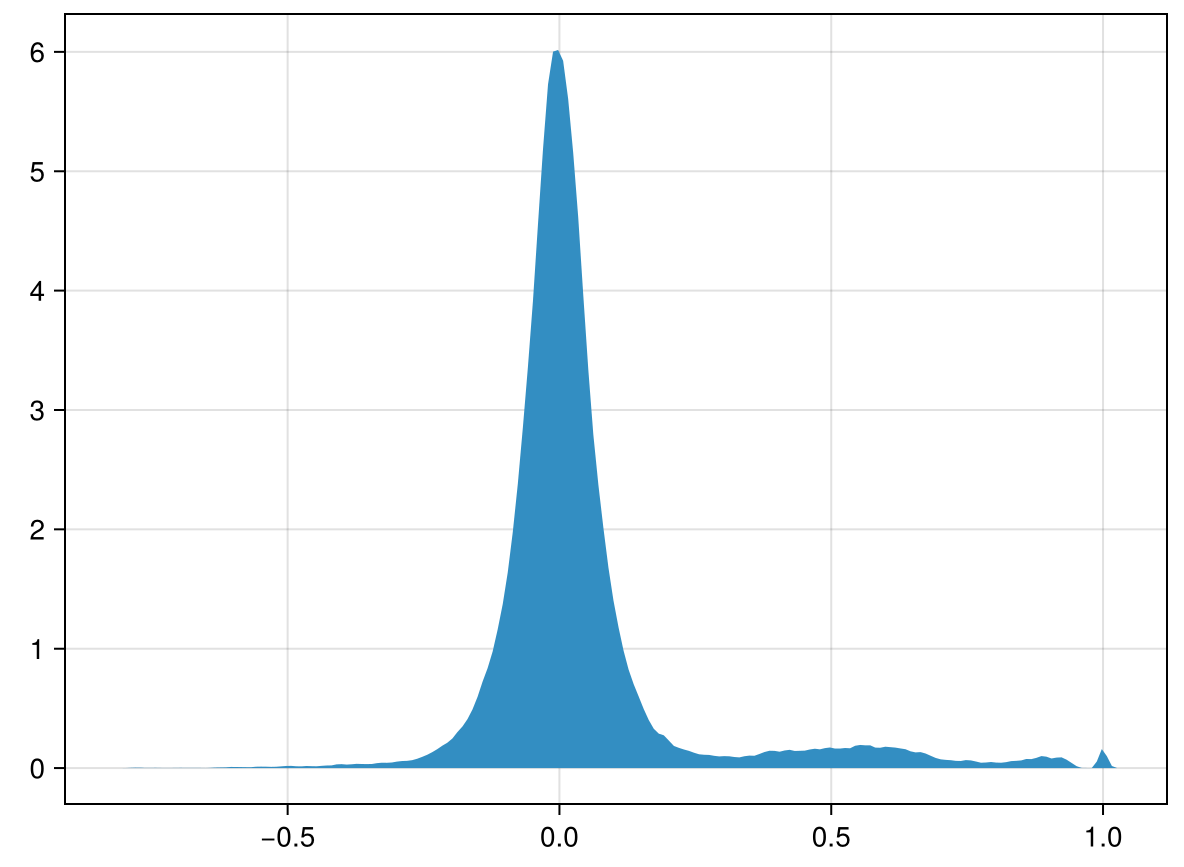
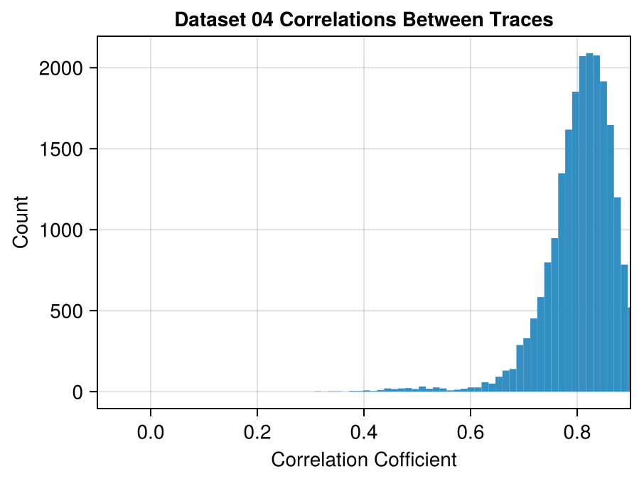
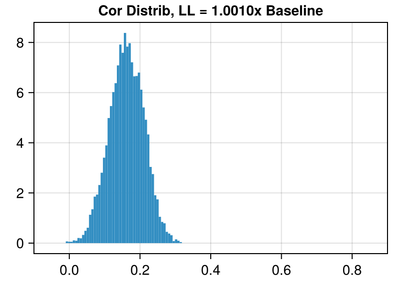
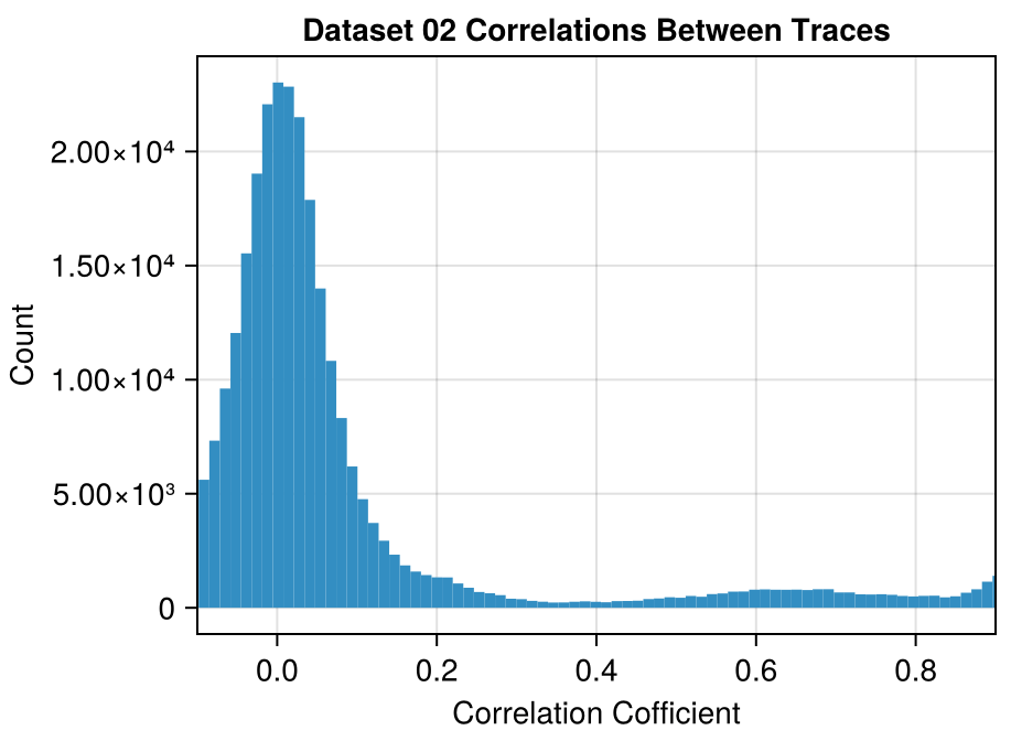
For each pair of traces \((i, j)\), compute the correlation between trace[i] and trace[j].
This gives us a square matrix consisting of all the pairwise correlations between different traces.
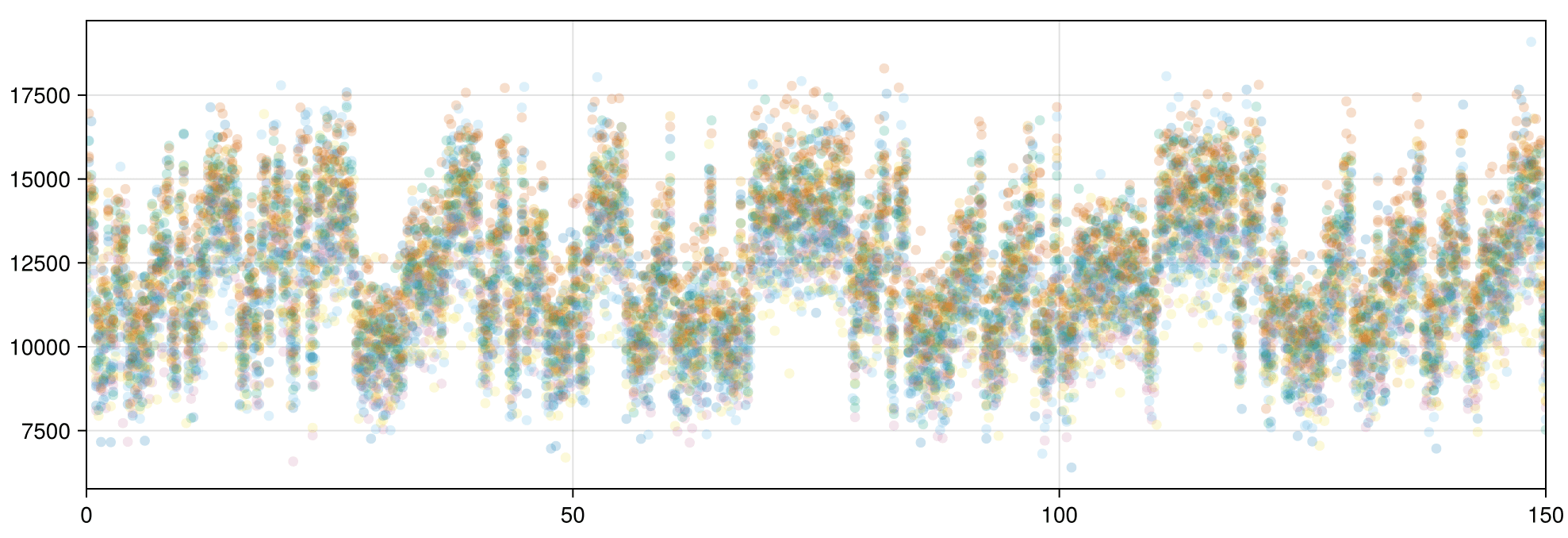
We can plot how often each correlation occurs to give us an idea of how much the different photon trajectories agree with each other.
(x-axis truncated for ease of viewing)
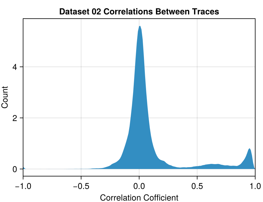
What's going on here?
In Dataset 02, there is a set of 67 traces where all traces in this set are correlated with each other at a coefficient of > 0.92.
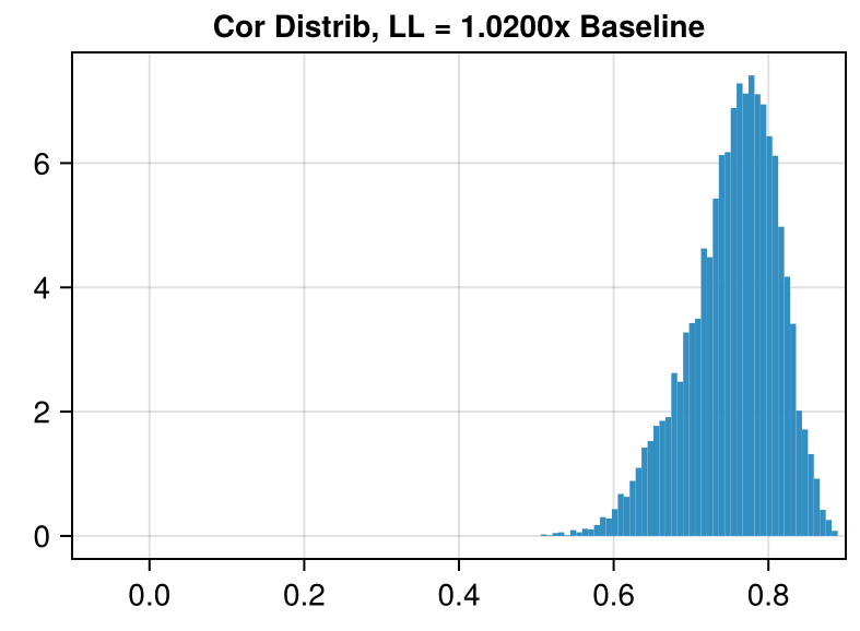
Even though the correlations in Dataset 04 are on average much higher, the largest set correlated mutually at > 0.92 only has 9 traces.
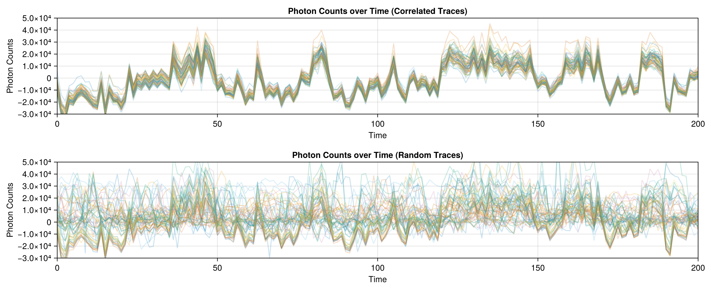
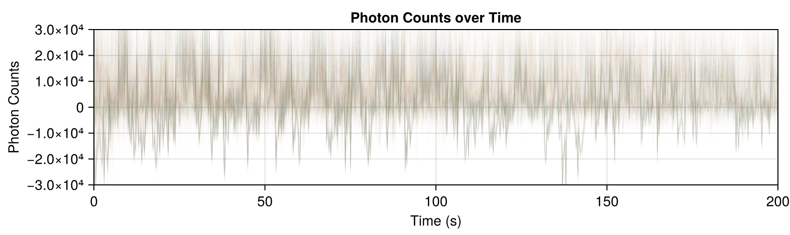
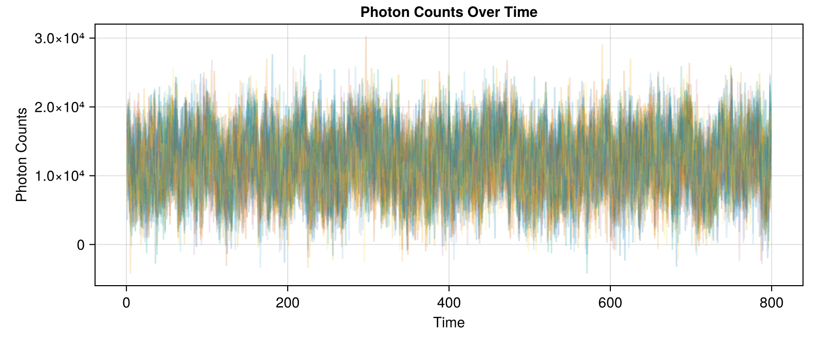
The correlated traces in Dataset 02 are visible even when plotting the data with high transparency: each line in the correlated set stacks to form a darker line.
Why, in a dataset where most traces are uncorrelated or weakly correlated, is there a small subset of traces that are this strongly correlated?
Should I try to throw some of them out? Weigh them more heavily when doing analysis? Pretend that there's nothing special about them?
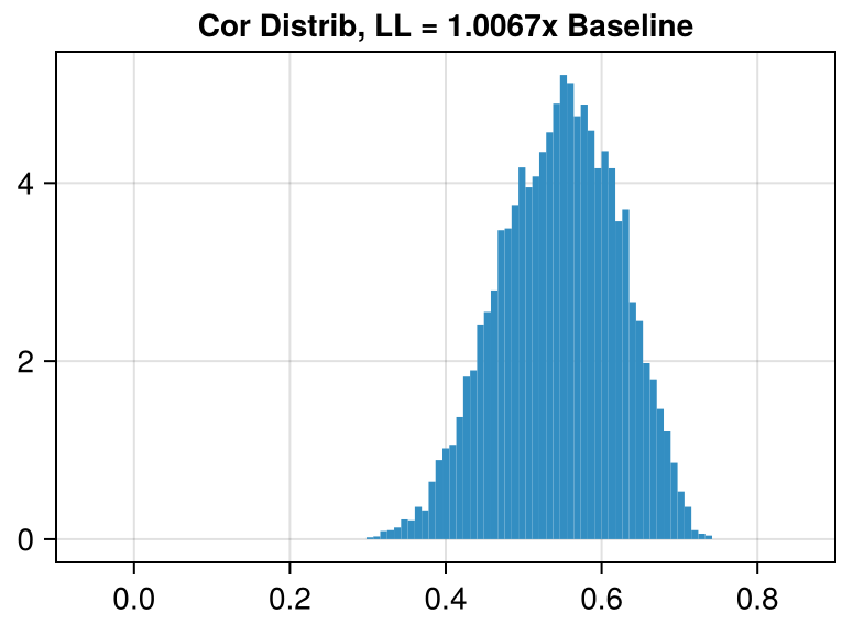
If we throw out the highly correlated traces, we can get rid of the peak of highly correlated traces....but now we have a bunch of uncorrelated data.
Filter by selecting connected components
Perfect 1.0 values caused by calculating self-correlations.
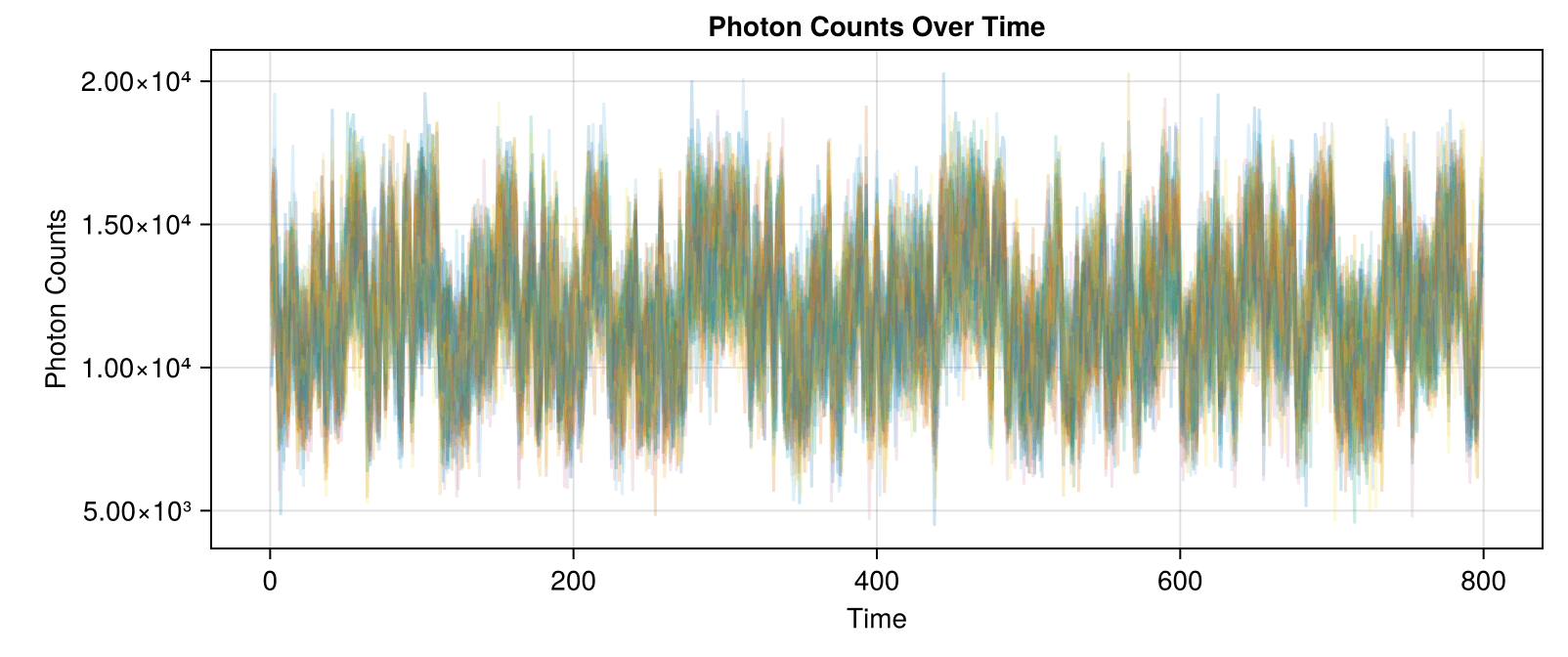
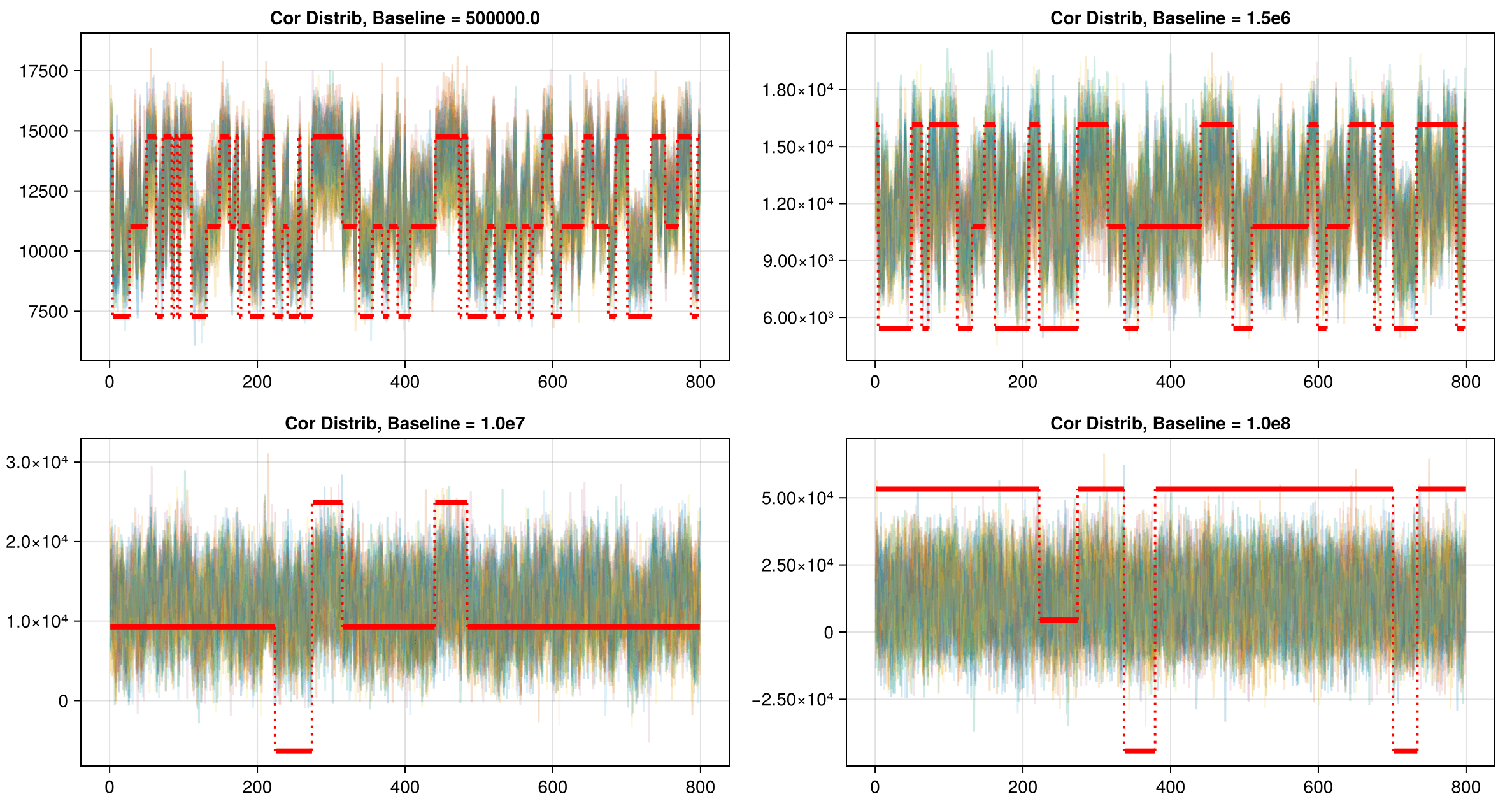
In synthetic data generated so far, background is ~500k, while signal is +10-15k over background.
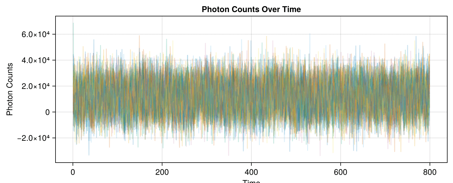
Leads to data and correlation plots like the following:
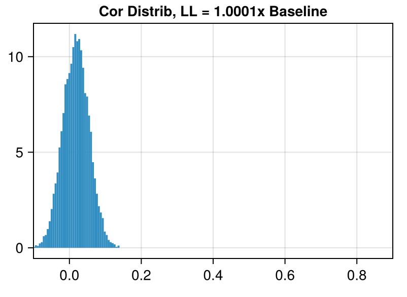
Synthetic data less correlated than experimental!
BG = 500,000
BG = 1,500,000
BG = 1,500,000
BG = 10,000,000
BG = 10,000,000
BG = 100,000,000
BG = 100,000,000
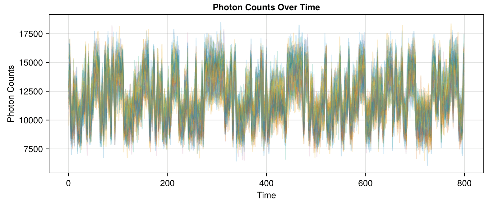
Dataset 02
Dataset 02 looks very similar to generation from a Poisson process where the background is 100,000,000 counts per interval and the signal is 100,010,000 counts per interval, a signal of one part in 1/10,000.
BG = 100,000,000
Dataset 02
DSet 02 is a signal with a mean of approximately 12,000 and a standard deviation of approximately 11,500.
Basically Random
Basically Random
Randomness comes from state-assignment algorithm, which uses a randomly-permuted k-means to assign initial clusters.
Changepoint-based analysis first tries to establish a single, canonical trajectory (basically placing a delta function on the space of possible trajectories) and then inferring entropy production from that.
Create state trajectories from various systems (e.g. two track, sfd, three state unidirectional, three state biased, three state unbiased).
Then noise them at different levels:
If HMMs can succeed in all three cases, then it is clearly much more capable than changepoints in high-noise environments.
Can BNP-step produce better changepoint assignments?
Probably not.
BUT it can give us posterior distributions over likely change points. Can we use this to compute our own ensemble entropy production?
First impression is that this seems like way too much computation.
Note: this procedure requires a state trajectory already: we need to know what state the system is in at any given time.
According to the instrument manual, there is an additional multiplicative noise factor which increases the variance of a steady-state signal by \( \sqrt{2} \) without affecting the mean.
To simulate this, since we know the actual mean of the distribution, subtract the observation from the mean and then multiply the difference appropriately, adding it back to the value.
function sample_scaled_poisson(p::Poisson)
	scale = sqrt(2)
    λ = mean(p)
    unscaled_sample = rand(p)
    delta = unscaled_sample - λ
    scaled_sample = λ + sqrt(scale) * delta
    return scaled_sample

    # Ensure non-negativity of sample, though
    # this should not be a problem in practice
    # for the scales we work at
    return max(scaled_sample, 0.0)
endBy Kevin Song


