Preferences and Utility
Christopher Makler
Stanford University Department of Economics
Econ 50: Lecture 4
🐟
🥥
Production Possibilities Fronier
Feasible
Lecture 3: Resource Constraints
Lecture 2: Production Functions
Labor
Fish
🐟
Capital
Coconuts
🥥
[GOODS]
⏳
⛏
[RESOURCES]
🐟
🥥
🙂
😀
😁
😢
🙁
Today: Preferences
How does Chuck rank
all possible combinations
of fish and coconuts?
Goal: find the best combination within his production possibilities set.
Feasible
Today's Agenda
Part 1: Modeling Preferences with Utility Functions
Part 2: Some "canonical" utility functions
Preferences: Definition and Axioms
Indifference curves
The Marginal Rate of Substitution
Utility Functions
Perfect Substitutes
Perfect Complements
Cobb-Douglas
Quasilinear
Preferences
Preferences: Ordinal Ranking of Options
Given a choice between option A and option B, an agent might have different preferences:
A \succ B
A \succeq B
A \sim B
A \preceq B
A \prec B
The agent strictly prefers A to B.
The agent strictly disprefers A to B.
The agent weakly prefers A to B.
The agent weakly disprefers A to B.
The agent is indifferent between A and B.
Sidebar: “Strictly" vs. “Weakly"
A \succ B
A \succeq B
The agent strictly prefers A to B.
The agent weakly prefers A to B.
2
3
4
5
6
x \ge 3
x \gt 3
Preference Axioms
Complete
Transitive
Any two options can be compared.
If \(A\) is preferred to \(B\), and \(B\) is preferred to \(C\),
then \(A\) is preferred to \(C\).
\text{For any options }A\text{ and }B\text{, either }A \succeq B \text{ or } B \succeq A
\text{If }A \succeq B \text{ and } B \succeq C\text{, then } A \succeq C
Together, these assumptions mean that we can rank
all possible choices in a coherent way.
Special case: choosing between bundles
containing different quantities of goods.
Preferences over Quantities
A=(4,3,6)
Example: “good 1” is apples, “good 2” is bananas, and “good 3” is cantaloupes:
🍏🍏🍏🍏
🍌🍌🍌
🍈🍈🍈🍈🍈🍈
B=(3,8,2)
🍏🍏🍏
🍌🍌🍌🍌🍌🍌🍌🍌
🍈🍈
General framework: choosing between anything
Special Case: Two Goods
Good 1 \((x_1)\)
Good 2 \((x_2)\)
Completeness axiom:
any two bundles can be compared.
Implication: given any bundle \(A\),
the choice space may be divided
into three regions:
preferred to A
dispreferred to A
indifferent to A
Indifference curves cannot cross!
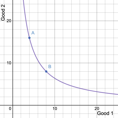
Marginal Rate of Substitution
X = (10,24)
🍏🍏
🍏🍏
🍏🍏
🍏🍏
🍏🍏
🍌🍌🍌🍌
🍌🍌🍌🍌
🍌🍌🍌🍌
🍌🍌🍌🍌
🍌🍌🍌🍌
🍌🍌🍌🍌
Y=(12,20)
🍏🍏
🍏🍏
🍏🍏
🍏🍏
🍏🍏
🍏🍏
🍌🍌🍌🍌
🍌🍌🍌🍌
🍌🍌🍌🍌
🍌🍌🍌🍌
🍌🍌🍌🍌
Suppose you were indifferent between the following two bundles:
Starting at bundle X,
you would be willing
to give up 4 bananas
to get 2 apples
Let apples be good 1, and bananas be good 2.
Starting at bundle Y,
you would be willing
to give up 2 apples
to get 4 bananas
MRS = {4 \text{ bananas} \over 2 \text{ apples}}
= 2\ {\text{bananas} \over \text{apple}}
Visually: the MRS is the magnitude of the slope
of an indifference curve
Utility Functions
How do we model preferences mathematically?
Approach: assume consuming goods "produces" utility
Production Functions
Labor
Fish
🐟
Capital
⏳
⛏
[RESOURCES]
Utility Functions
Utility
😀
[GOODS]
Fish
🐟
Coconuts
🥥
Representing Preferences with a Utility Function
u(a_1,a_2) > u(b_1,b_2)
u(a_1,a_2) \ge u(b_1,b_2)
u(a_1,a_2) = u(b_1,b_2)
u(a_1,a_2) \le u(b_1,b_2)
u(a_1,a_2) < u(b_1,b_2)
u(x_1,x_2)
"A is strictly preferred to B"
Words
Preferences
Utility
A \succ B
A \succeq B
A \sim B
A \preceq B
A \prec B
"A is weakly preferred to B"
"A is indifferent to B"
"A is weakly dispreferred to B"
"A is strictly dispreferred to B"
Suppose the "utility function"
assigns a real number (in "utils")
to every possible consumption bundle
We get completeness because any two numbers can be compared,
and we get transitivity because that's a property of the operator ">"
Marginal Utility
MU_1(x_1,x_2) = {\partial u(x_1,x_2) \over \partial x_1}
MU_2(x_1,x_2) = {\partial u(x_1,x_2) \over \partial x_2}
Given a utility function \(u(x_1,x_2)\),
we can interpret the partial derivatives
as the "marginal utility" from
another unit of either good:
Indifference Curves and the MRS
Along an indifference curve, all bundles will produce the same amount of utility
In other words, each indifference curve
is a level set of the utility function.
The slope of an indifference curve is the MRS. By the implicit function theorem,
MRS(x_1,x_2) = \frac{\partial u(x_1,x_2) \over \partial x_1}{\partial u(x_1,x_2) \over \partial x_2} = {MU_1 \over MU_2}
(Note: we'll treat this as a positive number, just like the MRTS and the MRT)
MRS = {MU_1 \over MU_2} =
u(x_1,x_2) = x_1x_2
MU_1 = {\partial u(x_1,x_2) \over \partial x_1} =
MU_2 = {\partial u(x_1,x_2) \over \partial x_1} =
A
B
Do we have to take the
number of "utils" seriously?
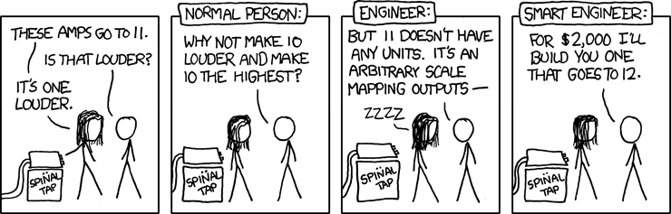
From XKCD:
Just like the "volume" on an amp, "utils" are an arbitrary scale...saying you're "11" happy from a bundle doesn't mean anything!
All we want to use utility functions for
is to describe preference orderings.
It doesn't matter that “utils" are nonsense.
As long as the utility function generates the correct indifference map,
it doesn't matter what the level of utility at each indifference curve is.
Transforming Utility Functions
Applying a positive monotonic transformation to a utility function doesn't affect
the way it ranks bundles.
u(x_1,x_2) = x_1^{1 \over 2}x_2^{1 \over 2}
\hat u(x_1,x_2) = 2x_1^{1 \over 2}x_2^{1 \over 2}
Example: \(\hat u(x_1,x_2) = 2u(x_1,x_2)\)
u(4,16) = 8
u(9,4) = 6
u(4, 16) = 2 \times 8 = 16
u(9,4) = 2 \times 6 = 12
Transformations and the MRS
Applying a positive monotonic transformation to a utility function doesn't affect
its MRS at any bundle (and therefore generates the same indifference map).
u(x_1,x_2) = x_1^{1 \over 2}x_2^{1 \over 2}
\hat u(x_1,x_2) = 2x_1^{1 \over 2}x_2^{1 \over 2}
MU_1 = {1 \over 2}x_1^{-{1 \over 2}}x_2^{1 \over 2}
MU_2 = {1 \over 2}x_1^{{1 \over 2}}x_2^{-{1 \over 2}}
MU_1 = x_1^{-{1 \over 2}}x_2^{1 \over 2}
MU_2 = x_1^{{1 \over 2}}x_2^{-{1 \over 2}}
MRS =
\displaystyle{= {x_2 \over x_1}}
\hat{MRS} =
\displaystyle{= {x_2 \over x_1}}
Example: \(\hat u(x_1,x_2) = 2u(x_1,x_2)\)
Transformations and the MRS
Applying a positive monotonic transformation to a utility function doesn't affect
its MRS at any bundle (and therefore generates the same indifference map).
u(x_1,x_2) = x_1^{1 \over 2}x_2^{1 \over 2}
\hat u(x_1,x_2) = {1 \over 2}\ln x_1 + {1 \over 2}\ln x_2
MU_1 = {1 \over 2}x_1^{-{1 \over 2}}x_2^{1 \over 2}
MU_2 = {1 \over 2}x_1^{{1 \over 2}}x_2^{-{1 \over 2}}
MU_1 = {1 \over 2x_1}
MU_2 = {1 \over 2x_2}
MRS =
\displaystyle{= {x_2 \over x_1}}
\hat{MRS} =
\displaystyle{= {x_2 \over x_1}}
Example: \(\hat u(x_1,x_2) = \ln(u(x_1,x_2))\)
Normalizing Utility Functions
One reason to transform a utility function is to normalize it.
This allows us to describe preferences using fewer parameters.
u(x_1,x_2) = a\ln x_1 + b\ln x_2
{1 \over a + b} u(x_1,x_2) = {a \over a + b}\ln x_1 + {b \over a + b}\ln x_2
\hat u(x_1,x_2) = \alpha \ln x_1 + (1 - \alpha)\ln x_2
[ multiply by \({1 \over a + b}\) ]
[ let \(\alpha = {a \over a + b}\) ]
= {a \over a + b}\ln x_1 + \left [1 - {a \over a + b}\right]\ln x_2
Desirable Properties of Preferences
We've asserted that all (rational) preferences are complete and transitive.
There are some additional properties which are true of some preferences:
- Monotonicity
- Convexity
- Continuity
- Smoothness
Monotonic Preferences: “More is Better"
\text{For any bundles }A=(a_1,a_2)\text{ and }B=(b_1,b_2)\text{, }A \succeq B \text{ if } a_1 \ge b_1 \text{ and } a_2 \ge b_2
\text{In other words, all marginal utilities are positive: }MU_1 \ge 0, MU_2 \ge 0
Nonmonotonic Preferences and Satiation
Some goods provide positive marginal utility only up to a point, beyond which consuming more of them actually decreases your utility.
Strict vs. Weak Monotonicity
Strict monotonicity: any increase in any good strictly increases utility (\(MU > 0\) for all goods)
Weak monotonicity: no increase in any good will strictly decrease utility (\(MU \ge 0\) for all goods)
Example: Pfizer's COVID-19 vaccine has a dose of 0.3mL, Moderna's has a dose of 0.5mL
Goods vs. Bads
\text{Good: }MU > 0
\text{Bad: }MU < 0
Convex Preferences: “Variety is Better"
Math background: "Convex combinations"
Convex Preferences: “Variety is Better"
Take any two bundles, \(A\) and \(B\), between which you are indifferent.
Would you rather have a convex combination of those two bundles,
than have either of those bundles themselves?
If you would always answer yes, your preferences are convex.
Concave Preferences: “Variety is Worse"
Take any two bundles, \(A\) and \(B\), between which you are indifferent.
Would you rather have a convex combination of those two bundles,
than have either of those bundles themselves?
If you would always answer no, your preferences are convex.
Common Mistakes about Convexity
1. Convexity does not imply you always want equal numbers of things.
2. It's preferences which are convex, not the utility function.
Other Desirable Properties
Continuous: utility functions don't have "jumps"
Smooth: marginal utilities don't have "jumps"
Counter-example: vaccine dose example
Counter-example: Leontief/Perfect Complements utility function
Well-Behaved Preferences
If preferences are strictly monotonic, strictly convex, continuous, and smooth, then:
Indifference curves are smooth, downward-sloping, and bowed in toward the origin
The MRS is diminishing as you move down and to the right along an indifference curve
Good 1 \((x_1)\)
Good 2 \((x_2)\)
"Law of Diminishing MRS"
Summary of Part I
Part I: properties of preferences,
and how preferences can be represented by utility functions.
Part II: see examples of utility functions,
and examine how different functional forms
can be used to model different kinds of preferences.
Take the time to understand this material well.
It's foundational for many, many economic models.
Econ 50 | 4 | Preferences and Utility
By Chris Makler


