Analyzing a Price Change
Christopher Makler
Stanford University Department of Economics
Econ 50: Lecture 14
Part I: Income and Substitution Effects
Break down overall effect
of a price change
into its component parts
How much does a price increase
hurt a consumer?
Part II: Welfare Analysis
More broadly: what is the relationship between money and utility?
Today's Agenda
Today's Agenda
Part 1: Income and Substitution Effects
Part 2: Welfare Analysis
Decomposing the effects of a price change
Finding the decomposition bundle
Income and substitution effects
Complements and Substitute
Relationship between utility & money
Compensating variation
Equivalent variation
Consumer's Surplus
Demand function: how does an optimal bundle change when prices or income changes?
If we want to know how best to implement a policy, we want to know why it changes.
For example: we could be interested in how far a cannonball travels, so we can aim it at a target.
To do this, a physicist would decompose its velocity
into the horizontal portion and vertical portion:
Two Effects
Substitution Effect
Effect of change in relative prices, holding utility constant.
Effect of change in real income,
holding relative prices constant.
Income Effect
Decomposition Bundle
Suppose that, after a price change,
we compensated the consumer
just enough to afford some bundle
that would give the same utility
as they had before the price change?
The Hicks decomposition bundle
is the lowest-cost bundle
that satisfies this condition.
Approach
TOTAL EFFECT
A
C
B
INITIAL BUNDLE
FINAL BUNDLE
DECOMPOSITION BUNDLE
SUBSTITUTION EFFECT
INCOME EFFECT
Income Offer Curve
Price Offer Curve
for a Good
Review: Offer Curves
Holding the prices of both goods constant,
show how the optimal bundle changes
as the consumer's income changes.
Holding the price of the other good
and consumer's income constant,
show how the optimal bundle changes
as the price of this good changes.
Offer curves are plotted in Good 1 - Good 2 space (along with budget lines and indifference curves)
pollev.com/chrismakler

A change in the price of good 1 will result in a ______ the price offer curve for good 1
and a ______ the income offer curve.
TOTAL EFFECT
A
C
B
INITIAL BUNDLE
FINAL BUNDLE
DECOMPOSITION BUNDLE
SUBSTITUTION EFFECT
INCOME EFFECT
Movement along POC
Shift of IOC
Movement along IOC
Hicks Decomposition
Hicks Decomposition Bundle
Suppose the price of good 1 increases from \(p_1\) to \(p_1^\prime\).
The price of good 2 (\(p_2\)) and income (\(m\)) remain unchanged.
Initial Bundle (A):
Solves
utility maximization
problem
Final Bundle (C):
Solves
utility maximization
problem
\max \ u(x_1,x_2)
\min \ p_1^\prime x_1 + p_2x_2
\text{s.t. }p_1x_1 + p_2x_2 = m
\text{s.t. }u(x_1,x_2) = U(A)
Decomposition Bundle (B):
Solves
cost minimization
problem
\max \ u(x_1,x_2)
\text{s.t. }p_1^\prime x_1 + p_2x_2 = m
"Compensated Budget Line"
The "compenated budget line" shows the budget line as if the consumer was given just enough money to achieve their initial utility at the new prices.
A consumer's compensated budget line:
"Compensated Budget Line"
If a consumer's preferences are well behaved, her compensated budget line
might lie below bundle A,
or pass through A, but cannot lie above A.
"Compensated Budget Line"
If a consumer's preferences are well behaved, her compensated budget line
might lie below bundle A,
or pass through A, but cannot lie above A.
Why? Because A could still be the cost-minimizing bundle, even at the new prices. But a budget line that passed above A
could not find the cost-minimizing bundle, because A would be cheaper!
In this example, \(p1\) and \(p_1\) started at 2 each, and then \(p_1\) rose to 8.
How would the diagram have been different if \(p_2\) had fallen to 0.5 instead?
pollev.com/chrismakler
In this example,
C was below and to the left of B.
What does that say about whether goods 1 and 2 are normal or inferior?
pollev.com/chrismakler
Complements and Substitutes (one last time)
Complements
Substitutes
When the price of good 1 goes up...
Net effect: buy less of both goods
Net effect: buy less good 1 and more good 2
Substitution effect: buy less of good 1 and more of good 2
Income effect (if both goods normal): buy less of both goods
Substitution effect dominates
Income effect dominates
= \begin{cases}\infty & \text{ if } x_1 < x_2 \\ 0 & \text{ if } x_1 > x_2 \end{cases}
-\infty
1
0
MRS = \left(x_2 \over x_1\right)^\infty
MRS = {x_2 \over x_1}
MRS = 1
r
u(x_1,x_2) = \min\{x_1,x_2\}
u(x_1,x_2) = x_1x_2
u(x_1,x_2) = x_1 + x_2
PERFECT
SUBSTITUTES
PERFECT
COMPLEMENTS
INDEPENDENT
PERFECT
SUBSTITUTES
u(x_1,x_2) = (x_1^r+x_2^r)^{1 \over r}
Constant Elasticity of Substitution (CES) Utility
MRS = \left(x_2 \over x_1\right)^{1-r}
u(x_1,x_2) = (x_1^r+x_2^r)^{1 \over r}
Constant Elasticity of Substitution (CES) Utility
MRS = \left(x_2 \over x_1\right)^{1-r}
-\infty
1
r
COMPLEMENTS: \(r < 0\)
SUBSTITUTES: \(r > 0\)
-1
MRS = \left(x_2 \over x_1\right)^2
{1 \over 2}
MRS = \left(x_2 \over x_1\right)^{1 \over 2}
u(x_1,x_2) = (x_1^{-1}+x_2^{-1})^{-1}
u(x_1,x_2) = \left(x_1^{1 \over 2} + x_2^{1 \over 2}\right)^2
Which of the following would be true if these goods were substitutes rather than complements?
pollev.com/chrismakler
Note: whether the goods are complements or substitutes has to do with the income and substitution effects on the good whose price has not changed.
(It's about how much you change your buying habits due to the change in another good.)
Hicks Decomposition: Worked Example
Hicks Decomposition Bundle
You have the utility function \(u(x_1,x_2) = x_1^{1 \over 2}x_2^{1 \over 2}\).
Suppose the price of good 1 increases from \(p_1 = 1\) to \(p_1^\prime = 4\).
The price of good 2 and income remain unchanged at \(p_2 = 1\) and \(m = 8\).
Initial Bundle (A):
Solves
utility maximization
problem
Final Bundle (C):
Solves
utility maximization
problem
\max \ u(x_1,x_2)
\min \ p_1^\prime x_1 + p_2x_2
\text{s.t. }p_1x_1 + p_2x_2 = m
\text{s.t. }u(x_1,x_2) = U(A)
Decomposition Bundle (B):
Solves
cost minimization
problem
\max \ u(x_1,x_2)
\text{s.t. }p_1^\prime x_1 + p_2x_2 = m
\max \ x_1^{1 \over 2}x_2^{1 \over 2}
\text{s.t. }x_1 + x_2 = 8
\min \ 4x_1 + x_2
\text{s.t. }x_1^{1 \over 2}x_2^{1 \over 2} = U(A)
\max \ x_1^{1 \over 2}x_2^{1 \over 2}
\text{s.t. }4 x_1 + x_2 = 8
(A) Solves utility maximization problem
(C) Solves utility maximization problem
(B) Solves cost
minimization problem
\max \ x_1^{1 \over 2}x_2^{1 \over 2}
\text{s.t. }x_1 + x_2 = 8
\min \ 4x_1 + x_2
\text{s.t. }x_1^{1 \over 2}x_2^{1 \over 2} = U(A)
\max \ x_1^{1 \over 2}x_2^{1 \over 2}
\text{s.t. }4 x_1 + x_2 = 8
Tangency condition:
Tangency condition:
Tangency condition:
{x_2 \over x_1} = 1
{x_2 \over x_1} = 4
Tangency condition:
Tangency condition:
Constraint:
Constraint:
Constraint:
x_1 + x_2 = 8
4 x_1 + x_2 = 8
x_1 = x_2
x_2 = 4x_1
{x_2 \over x_1} = 4
x_2 = 4x_1
Bundle B:
Bundle A:
Bundle C:
x_1 + \ \ \ \ \ = 8
x_1
4x_1 + \ \ \ \ \ \ = 8
4x_1
x_1^* = 4
(4,4)
(2,8)
(1,4)
x_1^* = 1
x_1^{1 \over 2}x_2^{1 \over 2} = 4
u(A) = 4^{1 \over 2}4^{1 \over 2} = 4
\text{s.t. }x_1^{1 \over 2}x_2^{1 \over 2} = 4
x_1^{1 \over 2}[\ \ \ \ \ \ \ \ ]^{1 \over 2} = 4
4x_1
2x_1 = 4
Hicks Decomposition Bundle
You have the utility function \(u(x_1,x_2) = x_1^{1 \over 2}x_2^{1 \over 2}\).
Suppose the price of good 1 increases from \(p_1 = 1\) to \(p_1^\prime = 4\).
The price of good 2 and income remain unchanged at \(p_2 = 1\) and \(m = 8\).
Initial Bundle (A):
Solves
utility maximization
problem
Final Bundle (C):
Solves
utility maximization
problem
Decomposition Bundle (B):
Solves
cost minimization
problem
\max \ x_1^{1 \over 2}x_2^{1 \over 2}
\text{s.t. }x_1 + x_2 = 8
\min \ 4x_1 + x_2
\text{s.t. }x_1^{1 \over 2}x_2^{1 \over 2} = U(A)
\max \ x_1^{1 \over 2}x_2^{1 \over 2}
\text{s.t. }4 x_1 + x_2 = 8
Bundle B:
Bundle A:
Bundle C:
(4,4)
(2,8)
(1,4)
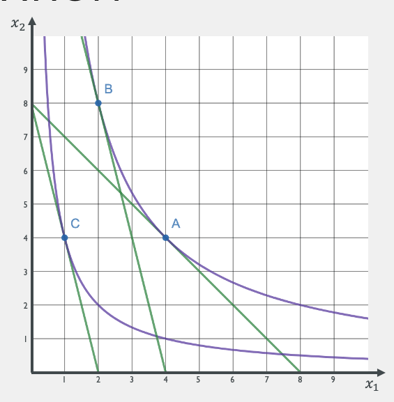
Hicks Decomposition Bundle
You have the utility function \(u(x_1,x_2) = x_1^{1 \over 2}x_2^{1 \over 2}\).
Suppose the price of good 1 increases from \(p_1 = 1\) to \(p_1^\prime = 4\).
The price of good 2 and income remain unchanged at \(p_2 = 1\) and \(m = 8\).
Initial Bundle (A): Solves utility maximization problem with the initial price
Final Bundle (C): Solves
utility maximization
problem with the new price
Decomposition Bundle (B):
Solves cost minimization
problem with the new price and initial utility
A=(4,4)
B=(2,8)
C=(1,4)
Econ 50 | Lecture 14
By Chris Makler
Econ 50 | Lecture 14
Analyzing a Price Change


