Using Consumer Theory to Analyze Policy Decisions
Christopher Makler
Stanford University Department of Economics
Econ 50: Lecture 16
Solving Climate Change in one Easy Step
- Climate change is real and caused in large part by burning fossil fuels.
- Transportation is a big part of the problem.
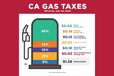
- A higher tax on gasoline would make people drive less, and have many other benefits. See Mankiw's Pigou Club Manifesto.
- Estimates vary, but $10/gallon seems about right.
but...
$10/gallon gas would hurt a lot of people, especially those with lower incomes who depend on a car to get to work
Can we give them a certain amount of money that would make them no worse off than they were before, to compensate them for the price increase?


Monday: Income and Substitution Effects
Break down overall effect
of a price change
into its component parts
How much does a price increase
hurt a consumer?
Today: Policy Analysis
How much utility can you buy with a certain amount of money?
How much money does a certain amount of utility cost?
This Week
Wednesday: Relationship between Money and Utility
How can we use policies that affect prices and income to improve outcomes?
Two Effects
Substitution Effect
Effect of change in relative prices, holding utility constant.
Effect of change in real income,
holding relative prices constant.
Income Effect
Decomposition Bundle
Suppose that, after a price change,
we compensated the consumer
just enough to afford some bundle
that would give the same utility
as they had before the price change?
The Hicks decomposition bundle
is the lowest-cost bundle
that satisfies this condition.
Approach
TOTAL EFFECT
INITIAL BUNDLE
FINAL BUNDLE
DECOMPOSITION BUNDLE
SUBSTITUTION EFFECT
INCOME EFFECT
Income Offer Curve
Price Offer Curve
for a Good
Review: Offer Curves
Holding the prices of both goods constant,
show how the optimal bundle changes
as the consumer's income changes.
Holding the price of the other good
and consumer's income constant,
show how the optimal bundle changes
as the price of this good changes.
Offer curves are plotted in Good 1 - Good 2 space (along with budget lines and indifference curves)
pollev.com/chrismakler

A change in the price of good 1 will result in a ______ the price offer curve for good 1
and a ______ the income offer curve.
TOTAL EFFECT
INITIAL BUNDLE
FINAL BUNDLE
DECOMPOSITION BUNDLE
SUBSTITUTION EFFECT
INCOME EFFECT
Movement along POC
Shift of IOC
Movement along IOC
Hicks Decomposition
Hicks Decomposition Bundle
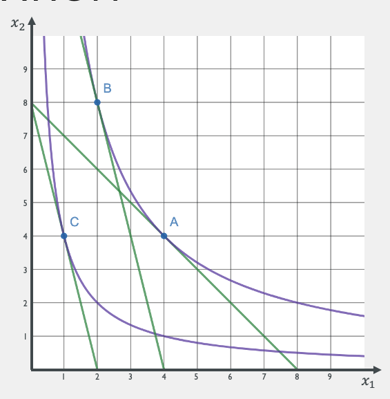
Suppose the price of good 1 increases from \(p_1\) to \(p_1^\prime\).
The price of good 2 (\(p_2\)) and income (\(m\)) remain unchanged.
Initial Bundle (A):
Solves
utility maximization
problem
Final Bundle (C):
Solves
utility maximization
problem
Decomposition Bundle (B):
Solves
cost minimization
problem
"Compensated Budget Line"
"Compensated Budget Line"

In this example, \(p1\) and \(p_1\) started at 2 each, and then \(p_1\) rose to 8.
How would the diagram have been different if \(p_2\) had fallen to 0.5 instead?
pollev.com/chrismakler

In this example,
C was below and to the left of B.
What does that say about whether goods 1 and 2 are normal or inferior?
pollev.com/chrismakler
Hicks Decomposition: Worked Example
Hicks Decomposition Bundle
You have the utility function \(u(x_1,x_2) = x_1^{1 \over 2}x_2^{1 \over 2}\).
Suppose the price of good 1 increases from \(p_1 = 1\) to \(p_1^\prime = 4\).
The price of good 2 and income remain unchanged at \(p_2 = 1\) and \(m = 8\).
Initial Bundle (A):
Solves
utility maximization
problem
Final Bundle (C):
Solves
utility maximization
problem
Decomposition Bundle (B):
Solves
cost minimization
problem
(A) Solves utility maximization problem
(C) Solves utility maximization problem
(B) Solves cost
minimization problem
Tangency condition:
Tangency condition:
Tangency condition:
Tangency condition:
Tangency condition:
Constraint:
Constraint:
Constraint:
Bundle B:
Bundle A:
Bundle C:
Hicks Decomposition Bundle
You have the utility function \(u(x_1,x_2) = x_1^{1 \over 2}x_2^{1 \over 2}\).
Suppose the price of good 1 increases from \(p_1 = 1\) to \(p_1^\prime = 4\).
The price of good 2 and income remain unchanged at \(p_2 = 1\) and \(m = 8\).
Initial Bundle (A):
Solves
utility maximization
problem
Final Bundle (C):
Solves
utility maximization
problem
Decomposition Bundle (B):
Solves
cost minimization
problem
Bundle B:
Bundle A:
Bundle C:
Hicks Decomposition Bundle
You have the utility function \(u(x_1,x_2) = x_1^{1 \over 2}x_2^{1 \over 2}\).
Suppose the price of good 1 increases from \(p_1 = 1\) to \(p_1^\prime = 4\).
The price of good 2 and income remain unchanged at \(p_2 = 1\) and \(m = 8\).
Initial Bundle (A): Solves utility maximization problem with the initial price
Final Bundle (C): Solves
utility maximization
problem with the new price
Decomposition Bundle (B):
Solves cost minimization
problem with the new price and initial utility

Welfare Effects of a Price Change
Consumer Theory Checklist
- Budget line / budget set
- Utility maximization
- Demand curve
- Price offer curve
- Income offer curve
- Hicks decomposition
- Cost minimization
Graphs / Representations
- Complements
- Substitutes
- Normal Goods
- Inferior Goods
- Income Effect
- Substitution Effect
- Compensating Variation
- Equivalent Variation
Concepts
- Utility-maximizing bundle given a budget constraint
- Ordinary (Marshallian) demand function
- Cost-minimizing bundle given a utility constraint
- Compensated (Hicksian) demand function
- Indirect utility function
- Expenditure function
Derivations
You should be able to perform this kind of analysis for any utility function,
including ones you haven't seen before (or seen before in this context).
Next Week:
From Consumers to Firms
- Monday: production and cost for a firm
- Wednesday: elasticity and revenue
- Friday: profit maximization
- Following Monday (11/11): Midterm 2
Econ 50 | Lecture 16
By Chris Makler
Econ 50 | Lecture 16
Analyzing a Price Change
- 956


