Welcome to Econ 51
Intertemporal Consumption
Christopher Makler
Stanford University Department of Economics
Econ 51: Lecture 1
Today's Agenda
Part 1: Course Overview
Part 2: Intertemporal Choice
Quick overview - read the syllabus!
Intertemporal budget line
Preferences over time
Optimal choice of saving and borrowing
Present value of multiple time periods
Introductions
Econ Department Peer Advising
Other Resources
VPTL Peer Tutoring
Three Central Themes
-
Time
-
Information
-
Equity and Efficiency
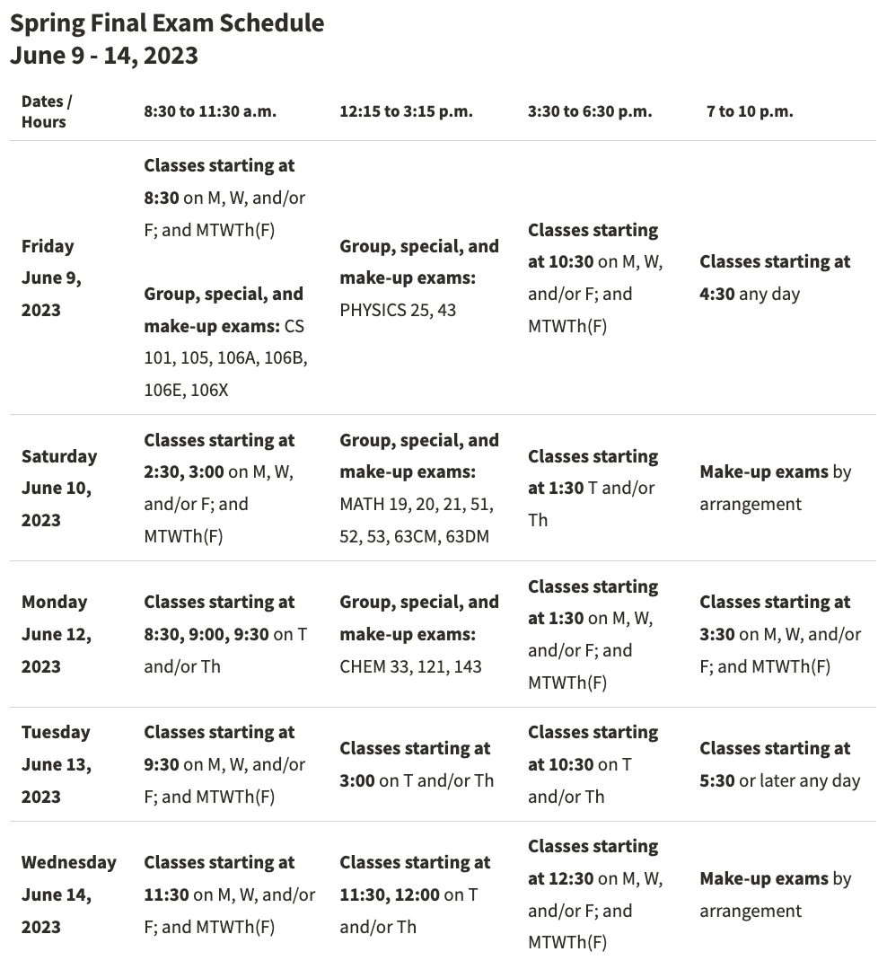
There's no way I'm going to ask you all to stay on campus until June 14.
And there's only one class in Week 10.
SO: We're just going to have the last test in that class of Week 10.
Online tests are terrible and invite cheating.
Weeks 1-3
Game Theory and Imperfect Competition
Tuesday 5/16
Exam on Unit II
Weeks 7-9
Efficiency and Equity
Quarter Rhythm
Weeks 4-6
The Economics of Information
Tuesday 4/25
Exam on Unit I
Tuesday 6/6
Exam on Unit III
Missing Exams
-
Exams are worth 65% of your grade. Due to multiple honor code violations during COVID, we are not giving students exams to take in isolation: if you miss an exam, for whatever reason, you miss the exam. We are having 3 exams to make it so that missing one exam is less of a big deal.
-
If you take all 3 exams:
-
lower midterm score is 15% of your grade
-
other two count for 25% of your grade
-
-
If you miss one of the midterms, we will re-weight the other two appropriately
-
If you miss more than one test, but have otherwise completed all the coursework, you will be given an Incomplete and will need to take any tests you missed in a future quarter.
Don't do this.
Tuesady, May 16
Exam 2
Tuesday, April 25
Exam 1
Tuesday, June 6
Exam 3
THESE ARE THE EXAM DATES.
DO NOT SCHEDULE VOLUNTARY TRAVEL THAT FORCES YOU TO MISS AN EXAM!!!
PUT THEM IN YOUR CALENDAR.
Course Web Sites
All content is posted/linked within Canvas.
Each lecture has its own module with everything you need to know about that lecture.
Please use Ed Discussions to ask questions (not email).
Please upload your homework to Gradescope by 8am the morning after it's due.
The Small Print
- Names and pronouns
- Students with documented disabilities
- Stanford University Honor Code
- Econ Department syllabus
- Humor gone wrong
Important?
Explained by Econ 50?
Time
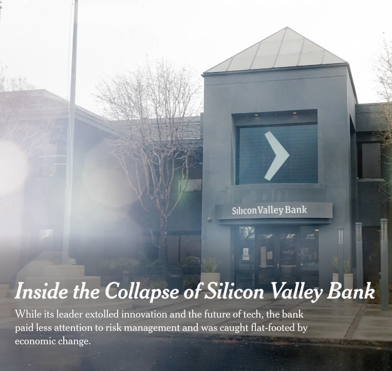
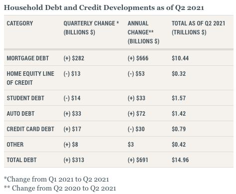
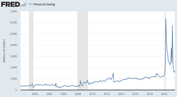
Saving and borrowing is a huge part of the U.S. economy.
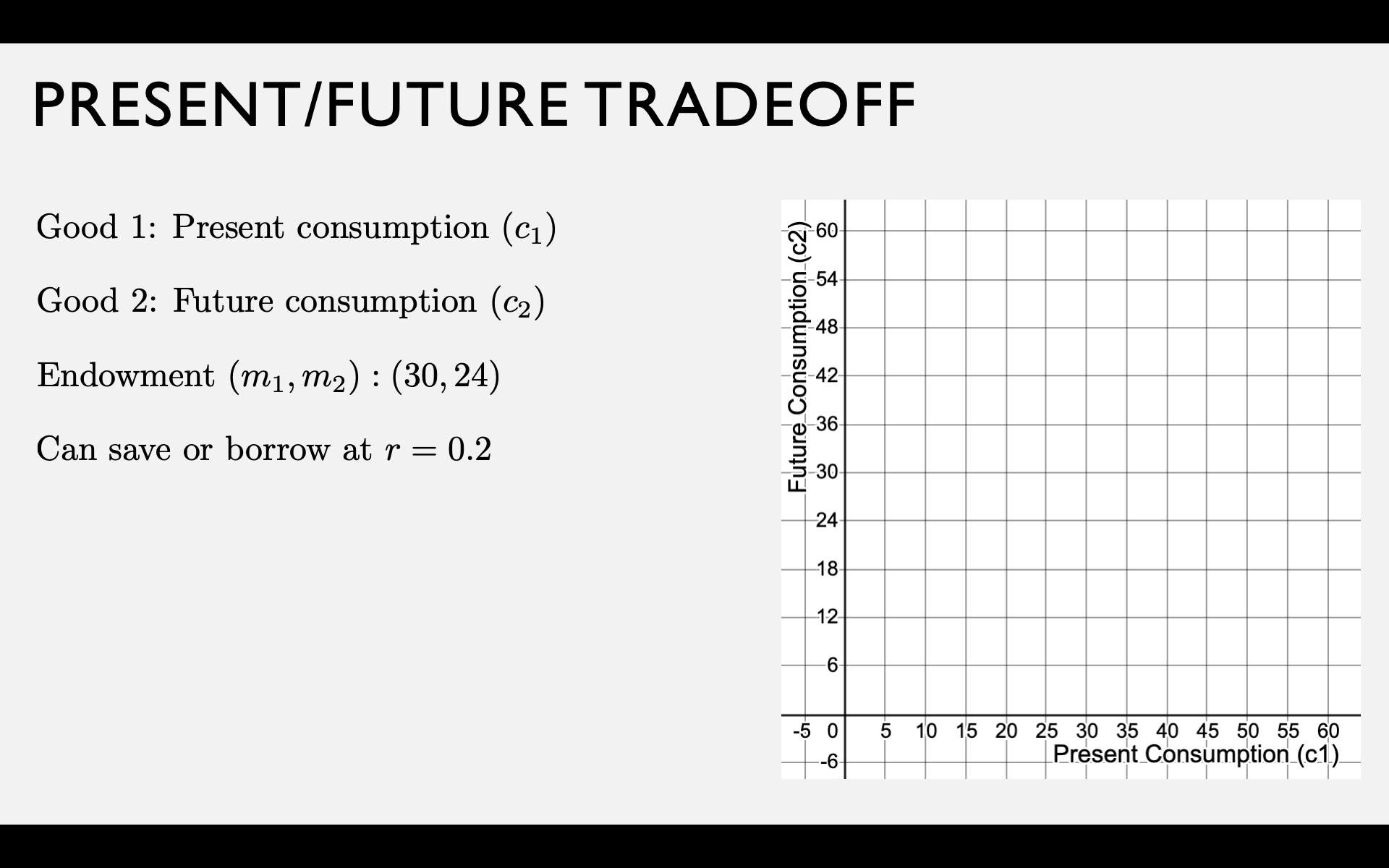
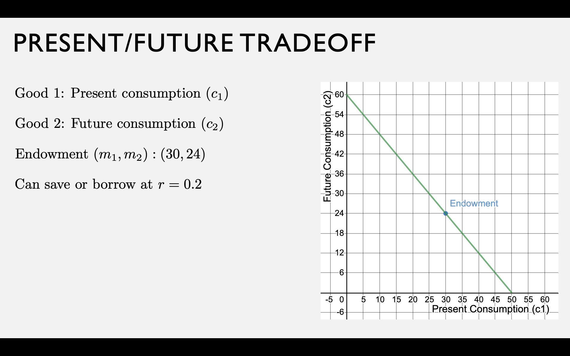
Present-Future Tradeoff
Your endowment is an income stream of \(m_1\) dollars now and \(m_2\) dollars in the future.
What happens if you don't consume all \(m_1\) of your present income?
Two "goods" are present consumption \(c_1\) and future consumption \(c_2\).
c_1 = m_1 - s
c_2 = m_2 + s
Let \(s = m_1 - c_1\) be the amount you save.
Saving and Borrowing with Interest
If you save at interest rate \(r\),
for each dollar you save today,
you get \(1 + r\) dollars in the future.
You can either save some of your current income, or borrow against your future income.
If you borrow at interest rate \(r\),
for each dollar you borrow today,
you have to repay \(1 + r\) dollars in the future.
c_1 = m_1 - s
c_2 = m_2 + (1+r)s
c_2 = m_2 + (1+r)(m - c_1)
(1+r)c_1 + c_2 = (1+r)m_1 + m_2
c_1 = m_1 + b
c_2 = m_2 - (1+r)b
c_2 = m_2 - (1+r)(c_1 - m_1)
(1+r)c_1 + c_2 = (1+r)m_1 + m_2
(1+r)c_1 + c_2 = (1 + r)m_1 + m_2
"Future Value"
1.2c_1 + c_2 = 1.2 \times 30 + 24
1.2c_1 + c_2 = 60
c_1 + \frac{c_2}{1+r} = m_1 + \frac{m_2}{1 + r}
"Present Value"
c_1 + \frac{c_2}{1.2} = 30 + \frac{24}{1.2}
c_1 + \frac{c_2}{1.2} = 50
Preferences over Time
u(c_1,c_2) = v(c_1)+\beta v(c_2)
v(c) = \text{“within-period" utility}
\beta = \text{“between-period" discount factor}
v(c) = \ln c
v(c) = c
u(c_1,c_2) = \ln c_1 + \beta \ln c_2
Examples:
v(c) = \sqrt{c}
u(c_1,c_2) = c_1 + \beta c_2
u(c_1,c_2) = \sqrt{c_1} + \beta \sqrt{c_2}
When to borrow and save?
u(c_1,c_2) = v(c_1)+\beta v(c_2)
MRS \text{ at endowment }= {v^\prime (m_1) \over \beta v^\prime (m_2)}
Save if MRS at endowment < \(1 + r\)
Borrow if MRS at endowment > \(1 + r\)
(high interest rates or low MRS)
(low interest rates or high MRS)
If we assume \(v(c)\) exhibits diminishing marginal utility:
MRS is higher if you have less money today (\(m_1\) is low)
and/or more money tomorrow (\(m_2\) is high)
MRS is lower if you are more patient (\(\beta\) is high)
Borrow or Save?
MRS(c_1,c_2) = {c_2 \over \beta c_1}
\text{MRS at endowment } =
\text{Price Ratio } =
\text{Example: }v(c_t) = \ln c_t \Rightarrow u(c_1,c_2) = \ln c_1 + \beta \ln c_2
m_1 = 30, m_2 = 24, r = 0.2
\text{Generic }m_1,m_2,r
\text{Borrow if } :
MRS(m_1,m_2) = {m_2 \over \beta m_1}
MRS(30,24) = {24 \over 30\beta}
1 + r
1.2
= {4 \over 5\beta}
= {6 \over 5}
>
{6 \over 5}
{4 \over 5\beta}
>
1 + r
MRS
\beta < {2 \over 3}
\text{Borrow if }\beta < \frac{2}{3}?
Optimal Bundle
\text{Example: }v(c_t) = \ln c_t \Rightarrow u(c_1,c_2) = \ln c_1 + \beta \ln c_2
Tangency condition:
Budget line:
MRS(c_1,c_2) = {c_2 \over \beta c_1}
m_1 = 30, m_2 = 24, r = 0.2
\text{Generic }m_1,m_2,r
{c_2 \over \beta c_1} = 1 + r
{c_2 \over \beta c_1} = 1.2
(1 + r)c_1 + c_2 = (1 + r)m_1 + m_2
1.2c_1 + c_2 = 1.2 \times 30 + 24
1.2c_1 + c_2 = 60
\Rightarrow c_2 = 1.2\beta c_1
\Rightarrow c_2 = (1+r)\beta c_1
(1 + r)c_1 + (1+r)\beta c_1 = (1 + r)m_1 + m_2
1.2c_1 + 1.2 \beta c_1 = 60
c_1^* = {1 \over 1 + \beta}(m_1 + {m_2 \over 1 + r})
c_2^* = {\beta \over 1 + \beta}((1 + r)m_1 + m_2)
c_1^* = {1 \over 1 + \beta} \times 50
c_2^* = {\beta \over 1 + \beta} \times 60
Supply of Savings and
Demand for Borrowing
At low interest rates, you'll "demand" funds for borrowing:
At high interest rates, you'll
"supply" funds for saving:
b(r) = c_1^*(r) - m_1
s(r) = m_1 - c_1^*(r)
Different Interest Rates
MRS > 1 + r
MRS < 1 + r
BORROW
SAVE
What if the interest rate is different for borrowing and saving?

c_2 = m_2 + (1 + r)(m_1 - c_1)
Inflation and Real Interest Rates
Suppose there is inflation,
so that each dollar saved can only buy
\(1/(1 + \pi)\) of what it originally could:
c_2 = m_2 + \left({1 + r\over 1 + \pi}\right)(m_1 - c_1)
Up to now, we've been just looking at
dollar amounts in both periods
\text{let }\rho = {1 + r \over 1 + \pi} - 1
c_2 = m_2 + (1 + \rho)(m_1 - c_1)
We call \(r\) the "nominal interest rate" and \(\rho\) the "real interest rate"
For low values of \(r\) and \(\pi\), \(\rho \approx r - \pi\)
c_1 + \frac{c_2}{1+r} = m_1 + \frac{m_2}{1 + r}
"Present Value" for two periods
Beyond Two Periods
If you save \(s\) now, you get \(x = s(1 + r)\) next period.
The amount you have to save in order to get \(x\) one period in the future is
s(1 + r) = x
s = {x \over 1 + r}
Remember how we got this...
If you save \(s\) now, you get \(x = s(1 + r)\) next period.
The amount you have to save in order to get \(x\) one period in the future is
s(1 + r) = x
s = {x \over 1 + r}
If you save for two periods, it grows at interest rate \(r\) again, so \(x_2 = (1+r)(1+r)s = (1+r)^2s\)
Therefore, the amount you have to save in order to get \(x_2\) two periods in the future is
s(1 + r)^2 = x_2
s = {x_2 \over (1 + r)^2}
If you save for two periods, it grows at interest rate \(r\) again, so \(x_2 = (1+r)(1+r)s = (1+r)^2s\)
Therefore, the amount you have to save in order to get \(x_2\) two periods in the future is
s(1 + r)^2 = x_2
s = {x_2 \over (1 + r)^2}
If you save for \(t\) periods, it grows at interest rate \(r\) each period, so \(x_t = (1+r)^ts\)
Therefore, the amount you have to save in order to get \(x_t\), \(t\) periods in the future, is
s(1 + r)^t = x_t
s = {x_t \over (1 + r)^t}
Therefore, the amount you have to save in order to get \(x_t\), \(t\) periods in the future, is
s(1 + r)^t = x_t
s = {x_t \over (1 + r)^t}
We call this the present value of a payoff of \(x_t\)
PV(x_t) = {x_t \over (1 + r)^t}
The present value of an income stream is the sum of the present values in each period:
PV(x_0,x_1,x_2) = x_0 + {x_1 \over 1 + r} + {x_2 \over (1 + r)^2}
Evaluating Infinite Payoffs
V(\pi_0,\pi_1,\pi_2, \cdots) = \pi_0 + {\pi_1 \over 1 + r} + {\pi_2 \over (1 + r)^2} + \cdots
V(x,x,x, \cdots) = x + {x \over 1 + r} + {x \over (1 + r)^2} + \cdots
The present value of a stream of payoffs
(\(\pi_0\) now, \(\pi_1\) in the next period, \(\pi_2\) two periods from now, etc)
may be given by the sum
The present value of a stream of payoffs of \(x\) in every period is
x + {x \over r}
Value of getting payoff \(x\) forever, starting now:
Value of getting payoff \(z\) forever, starting next period:
Value of getting payoff \(y\) now and then payoff \(z\) forever after:
{z \over r}
y + {z \over r}
Application: Social Cost of Carbon
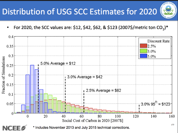
Obama Admin: $45
Uses a 3% discount rate; includes global costs
Trump Admin: less than $6
Uses a 7% discount rate; only includes American costs
PV of $1 Trillion in 2100:
$86B for Obama, $4B for Trump
To Do Before Next Class
Be sure you've filled out the section survey.
Read chapters 1-5 of Watson and do the quiz!
Econ 51 | Spring 23 | 1 | Welcome and Intertemporal Consumption
By Chris Makler


