Temporal Relational Ranking for Stock Prediction
Feng et al.
Motivation
- Most methods are either time series or cross-sectional
- Most optimized for classification or regression
Objective
- Tailor deep learning models for stock ranking
- Capture stock relations in a time-sensitive manner
Results
- New component: Temporal Graph Convolution (TGC)
-
Novel architecture: Relational Stock Ranking (RSR)
- Combine LSTM with TGC
- Jointly models temporal evolution and relation network of stocks
- Back-testing on NASDAQ and NYSE
- Beats benchmarks and SFM model
Background
Ranking as a Target
- Classification and regression may be suboptimal
- Ranking selects stocks with highest expected revenue
Ranking as a Target
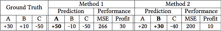
- Method 2: \(\downarrow\) MSE, \(\downarrow\) profit
- Method 1: picked the biggest change,
\(\uparrow\) MSE, \(\uparrow\) profit
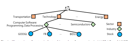
Stock Relations
- Three types of relations:
- Industry
- First Order
- Second Order
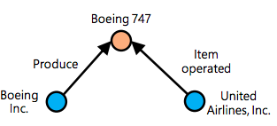
- Relations are stated as (subject; predicate; object)
Stock Relations
- Industry:
- NASDAQ and NYSE classify each stock into a sector and industry
- (GOOGL; Computer Software: Programming, Data Processing; FB)
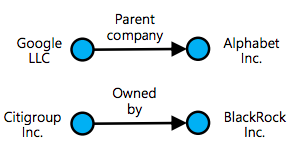
Stock Relations
- First and Second Order:
- Data from Wikidata
- Tens of millions of objects
- Hundreds of millions of statements
- (Alphabet, Inc.; founded by; Larry Page)
Stock Relations
- First Order:
- Company \(i\) has a first order relation with \(j\) if there is a statement with \(i\) as the subject and \(j\) as the object
- (Citigroup Inc.; owned by; BlackRock Inc.)
Stock Relations
- Second Order:
- Company \(i\) has a second order relation with \(j\) if they have statements sharing the same object
Stock Relations
Previous/Component Models
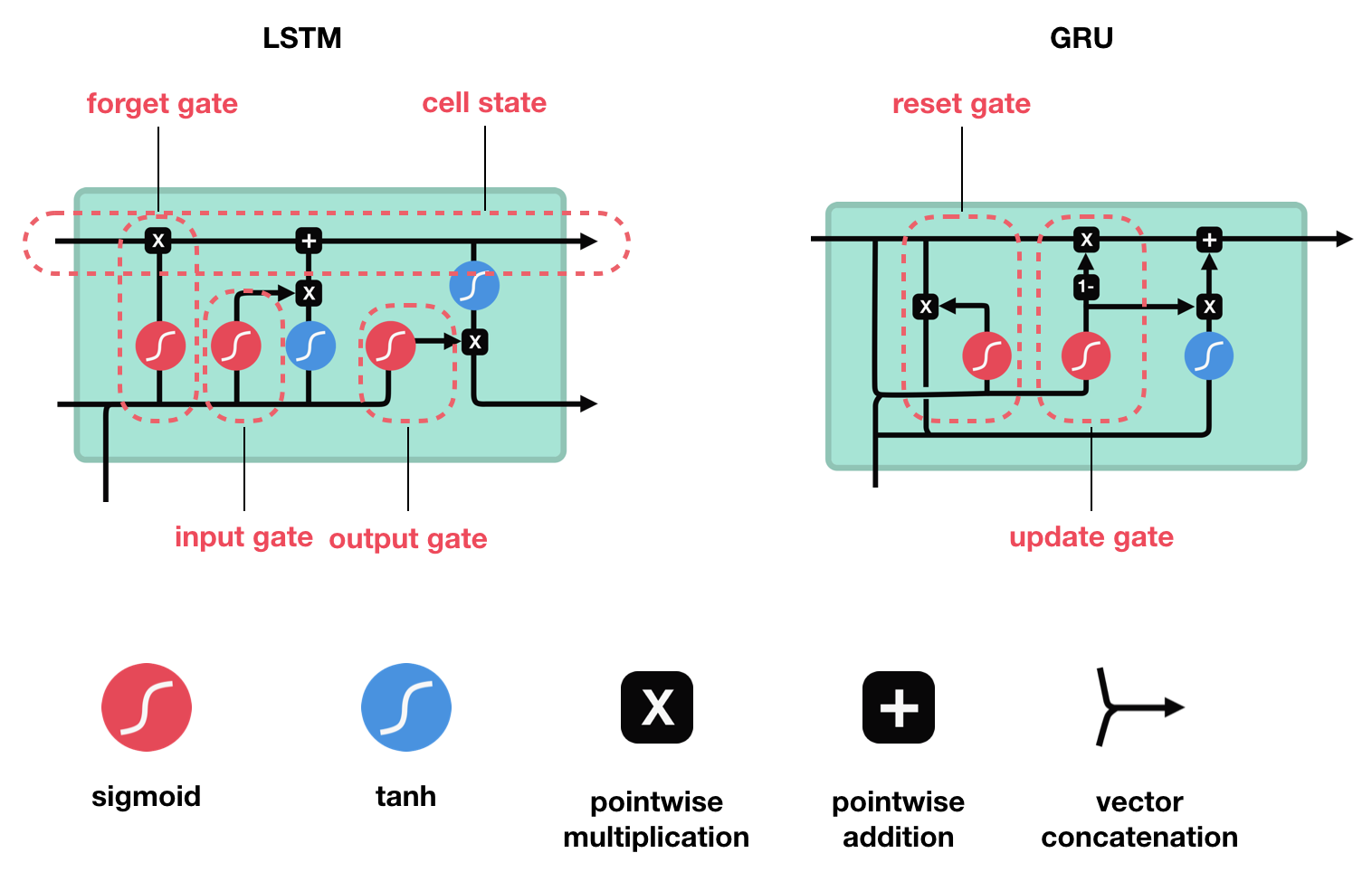
Long Short Term Memory
(LSTM)
Graph-based Learning
- Minimize objective function \(\Gamma=\Omega+\lambda\Phi\)
- \(\Omega\): task specific loss
- \(\Phi\): graph regularization term; smooths prediction over graph
\[\Phi=\sum_{i=1}^N\sum_{j=1}^N \text{strength of smoothness}_{ij}\cdot \text{smoothness}_{ij}\]
Graph-based Learning
\[\Phi=\sum_{i=1}^N\sum_{j=1}^N \text{strength of smoothness}_{ij}\cdot \text{smoothness}_{ij}\]
- Strength of smoothness= \(g(x_i,x_j)\) = similarity between feature vectors
- i.e., edge weight
Graph-based Learning
\[\Phi=\sum_{i=1}^N\sum_{j=1}^N \text{strength of smoothness}_{ij}\cdot \text{smoothness}_{ij}\]
- smoothness=\(||\frac{f(x_i)}{\sqrt{D_{ii}}} - \frac{f(x_j)}{\sqrt{D_{jj}}}||^2\)
- \(D_{ii}\): degree of node \(i\)
- Enforces that similar nodes have similar predictions
Graph Convolutional Networks
- Combine smoothness assumption with CNNs
- Cannot directly apply convolution onto adjacency matrix
- Solution: Use spectral convolutions
Graph Convolutional Networks
\[f(F,X)=UFU^TX\]
- \(f\): filtering operation of convolution
- \(F\): diagonal matrix parameterizing convolution
- \(U\): eigenvector matrix of graph Laplacian matrix \(L\)
- \(L=U\Lambda U^T=D^{-1/2}(D-A)D^{-1/2}\)
Graph Convolutional Networks
\[f(F,X)=UFU^TX\]
- Approximate equation with Chebyshev polynomials of order \(k=1\) (proven sufficient in previous work)
- Reduces to \(f(F,X)=AX\)
- Elements of A: \(A_{ij}=g(x_i,x_j)\)
- Inject convolution into a fully connected layer as \(A(XW+b)\)
New Model
Relational Stock Ranking
- Input:
- \(X^t=[x^{t-S+1},\dots,x^t]^T\in \R^{S\times D}\)
- sequential input features of a specific stock
- sequence length \(S\); \(D\) features
- \(\mathcal X^t\in \R^{N\times S\times D}\)
- collected sequential features of all \(N\) stocks
- Target: \(\hat r^{t+1}=f(\mathcal X^t)\)
- ranking-aware 1-day return
Relational Stock Ranking
- Relations of two stocks:
- \(K\) types of relations
- Encode pairwise relation between two stocks as a multi-hot binary vector \(a_{ij}\in \R^k\)
- Relation of all stocks:
- \(\mathcal A \in \R^{N\times N\times K}\)
- \(i\)-th row, \(j\)-th column is \(a_{ij}\)
Relational Stock Ranking
- Three Layers:
- Sequential Embedding Layer
- Relational Embedding Layer
- Prediction Layer
Relational Stock Ranking
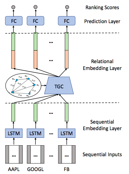
Sequential Embedding Layer
- Intuitive to first regard the historical status of a stock
- First apply a sequential embedding layer
- Choose LSTM since captures long-term dependency
- ex: interest rates
Sequential Embedding Layer
- Take last hidden state \(h_i^t\)
- Set it as sequential embedding \(e_i^t=h_i^t\)
- \(E^t=LSTM(\mathcal X^t)=[e_1^t,\dots,e_N^t]^T\in \R^{N\times U}\)
- \(U\): number of hidden units in LSTM
Relational Embedding Layer
- New component of neural network modeling: Temporal Graph Convolution
- Generates relational embeddings \(\bar E^t\in \R^{N\times U}\)
- These are time-sensitive (dynamic)
- Key technical contribution of this work
- We will build up the model intuitively
Relational Embedding Layer
- Uniform Embedding Propagation
- From link analysis
\[\overline{e_i^t} = \sum_{\{j|sum(a_ji)>0\}} \frac{1}{d_j}e_j^t\]
- Only stocks that have at least one relation are used
- \(d_j\): number of stocks satisfying the condition
Relational Embedding Layer
2. Weighted Embedding Propagation
- Different relations may have different impacts
\[\overline{e_i^t} = \sum_{\{j|sum(a_ji)>0\}} \frac{g(a_{ji})}{d_j}e_j^t\]
- g: Relation-strength function
- Aims to learn impact strength of relations in \(a_{ji}\)
Relational Embedding Layer
3. Time-aware Embedding Propagation
- Relation-strength may evolve over time
\[\overline{e_i^t} = \sum_{\{j|sum(a_ji)>0\}} \frac{g(a_{ji},e_i^t,e_j^t)}{d_j}e_j^t\]
- Includes temporal and stock information
Relational Embedding Layer
- Two designs of \(g\):
- Explicit modeling
- Implicit modeling
Relational Embedding Layer
- Explicit modeling:
g(a_{ji},e_i^t,e_j^t)=e_i^{t^T}e_j^t\times \phi(w^Ta_{ji}+b)
similarity
relation importance
- \(w\in\R^K,b\): model parameters to be learned
- \(\phi\): leaky rectifier activation function
Relational Embedding Layer
- Implicit modeling:
g(a_{ji},e_i^t,e_j^t)=\phi(w^T[e_i^{t^T},e_j^{t^T},a_{ji}^T]^T+b)
- \(w\in\R^{2U+K},b\): learned
- Learn both similarity and relation importance
- \(g\) is then normalized through a softmax function
Relational Embedding Layer
- Connection with graph-based learning:
- Embedding propagation equivalent to GCN at time \(t\)
- Proof omitted
- GCN must have fixed adjacency matrix
Prediction Layer
- Feed both sequential embeddings and revised relational embeddings into a fully connected layer to predict rank-aware returns
Prediction Layer
- Proposed objective function:
l(\hat r^{t+1},r^{t+1})=||\hat r^{t+1}-r^{t+1}||^2+\alpha \sum_{i=0}^N\sum_{j=0}^N \max\{0,-(\hat r_i^{t+1}-\hat r_j^{t+1})(r_i^{t+1}-r_j^{t+1})\}
- First term: SSE
- punishes difference between ground-truth and prediction
- Second term: pair-wise max-margin loss
- Encourages predicted ranking scores of stock pair to have the same relative order as ground-truth
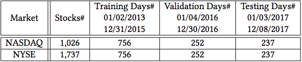
Data
Sequential Data
- Source: Google Finance
- Historical price data from NASDAQ and NYSE
- NASDAQ more volatile, NYSE more stable
- Filter stocks:
- Traded on at least 98% of days
- Never been traded less than $5.00
Historical Price Data
Historical Price Data
- \(p_i^t\): closing price of stock \(i\) on day \(t\)
- Normalized by max price of stock \(i\)
- Ground truth: \(r_i^{t+1}=(p_i^{t+1}-p_i^t)/p_i^t\)
- Calculate 5, 10, 20, 30 day moving averages of returns
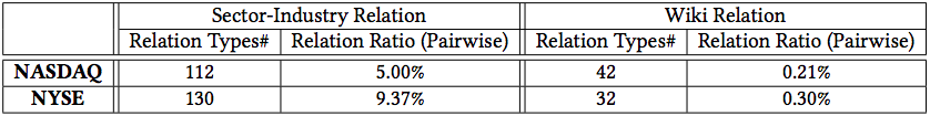
Stock Relation Data
- Sector-industry relations: NASDAQ and NYSE
- Company-based relations: Wikidata
Experiment
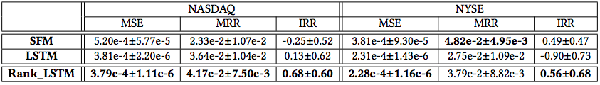
Three Metrics:
- Mean Squared Error (MSE)
- Want smaller value of MSE (\(\geq 0\))
- Mean Reciprocal Rank (MRR)
- Take average of reciprocal rank of selected stock
- Want larger value of MRR (\([0,1]\))
- Cumulative Investment Return Ratio (IRR)
- Want larger value of IRR
Experimental Setting
- Market close on day \(t\): predict a ranking list and buy the highest ranked stock
- Market close on day \(t+1\): sell the stock
Experimental Setting
Assumptions:
- Same amount of money spent every day
- Market liquid enough to buy stock at the closing price on day \(t\)
- Liquid enough to sell at closing price on day \(t+1\)
- Transaction costs ignored
Methods
- SFM: Fourier signal deep learning
- LSTM: regression target
- Rank_LSTM: rank target
- GBR: add graph regularization term to Rank_LSTM
- GCN: static graph convolution
- RSR_E: explicitly modeled RSR
- RSR_I: implicitly modeled RSR
Methods
- Grid search validation
- Adam optimizer, learning rate 0.001
Three Research Questions
- How does ranking compare to classification or regression? Can RSR outperform SOTA solutions?
- Do stock relations enhance the neural network-based solution? Does TGC outperform GBR or GCN?
- How does our proposed RSR solution perform under different back testing strategies?
Q1: Rank
- Rank_LSTM outperforms SFM and LSTM in IRR
- Fails to beat in all metrics
- Could be because there is a tradeoff between accurately predicting value and order
- High variance
- Picking one stock volatile
-
LSTM performs unexpectedly bad on the NYSE
- Can do better with different parameters (snooping)
Q1: Rank
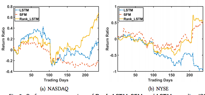
Q1: Rank
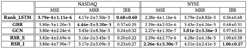
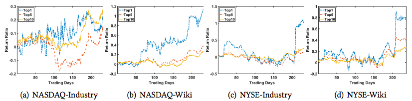
Q2: Relations: Industry
- Industry relations more valuable on NYSE than NASDAQ
- NYSE less volatile, industry relations are long-term
- On NYSE, all relational methods outperform Rank_LSTM
- On NYSE, RSR_E and RSR_I are top two methods
- Performance across metrics again inconsistent
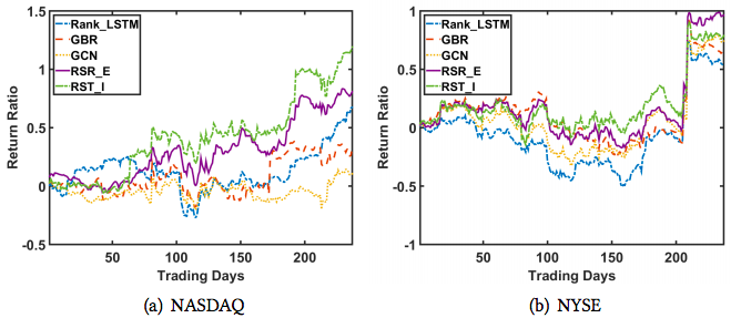
- On NYSE, much of gains achieved on days 206 and 209
- Importance of accurately doing rank and size
Q2: Relations: Industry
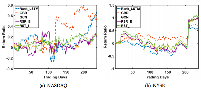
Q2: Relations: Industry
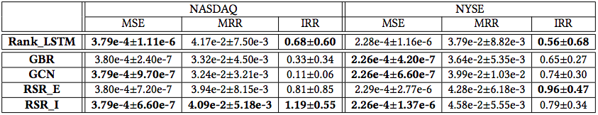
Q2: Relations: Wiki
-
RSR_E and RSR_I achieve best IRR performance
- Especially on NYSE
Q2: Relations: Wiki
Q2: Relations: Wiki
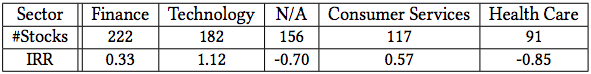
Q2: Relations: Sector-wise
- Is the performance sensitive to sectors?
- Back-tested each sector separately on NASDAQ
- Only technology produced an acceptable IRR
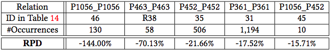
Q2: Relations: Types of Wiki
- Compared performance when a type of relation was removed
- Top 5 factors:
- Product or material produced
- Member of
- Industry
- Part of
- Product or material produced; Industry
Q2: Relations: Types of Wiki
Q2: Brief Conclusion
- Considering stock relations helpful for stock ranking, especially on stable markets
- Proposed TGC is promising model for stock relations
- Important to consider appropriate relations suitable for the target market
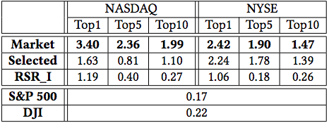
Q3: Strategy
- Three strategies: Top1, Top5, Top10
- Equally split budget among stocks
-
Top1>Top5>Top10
- If ranking algorithm good, then should put all money on stock with highest expected return
- RSR_I continues to do poorly in NASDAQ-Industry
Q3: Strategy
Q3: Strategy: Comparison to Benchmarks
- Compare strategy to S&P 500 and DJIA
- Also formulate two ideal versions of strategies:
- Market: select stocks with highest return ratio from the whole market
- Selected: select stocks with highest return ratio from the set of stocks traded by RSR_I
Q3: Strategy: Comparison to Benchmarks
Conclusion
- Demonstrated potential of learning-to-rank methods
- Proposed RSR framework with novel TGC component
- Outperforms indicies and SOTA methods
Future Work
- Explore more advanced learning-to-rank techniques
- Integrate risk management
- Investigate other strategies
- buy-hold-sell (long)
- borrow-sell-buy (short)
- Integrate alternative data
- News/social media
- Explore TGC in other fields
Analysis
- Trading strategy seems unlikely
- No reports on statistical significance
- Not sure why prices were normalized if in return space
- Would like to see sector relations as well
- Would like to see all types of relations at once
- Everything available on github
Temporal Relational Ranking
By Connor Chapin
Temporal Relational Ranking
Presentation on "Efficient Estimation of Word Representations in Vector Space"