Autoencoder Asset Pricing Models
Gu, Kelly, and Xiu
Motivation
- The IPCA model (a latent factor conditional asset pricing model) is powerful.
- However, it assumes the factor exposures are a linear function of the covariates.
- Existing literature suggests their relationship might be nonlinear.
Objective
- Create a nonlinear version of IPCA using autoencoders
Results
- Reduces out-of-sample pricing errors (predictive \(R^2\))
- Imposes economic restriction of no-arbitrage (no intercept)
Background
A model of returns
\[r_{i,t+1}=\alpha_{i,t}+\beta'_{i,t}f_{t+1}+\epsilon_{i,t+1}\]
- \(r_{i,t+1}\): return for stock \(i\) at time \(t+1\)
- \(f_{t+1}\): systemic risk factors at time \(t+1\)
- \(\beta'_{i,t}\): exposure of stock \(i\) at \(t+1\) to systemic risk factors
- \(\alpha_{i,t}\): intercept term (perhaps set to 0)
- \(\epsilon_{i,t+1}\): error
A model of returns
\[r_{i,t+1}=\alpha_{i,t}+\beta'_{i,t}f_{t+1}+\epsilon_{i,t+1}\]
-
\(f_{t+1}\): systemic risk factors at time \(t+1\)
- These are the "factors" in a factor model
- Systemwide: no \(i\) subscript
- Can be pre-specified or latent
- We will use latent factors
IPCA
- From "Characteristics are covariances" by KPS
- Idea: characteristics proxy for exposure to risk factors
- Momentum, volatility, bid-ask spread
- Conditional exposures: \(\beta(z_{i,t})'=z'_{i,t}\Gamma_\beta\)
- \(z_{i,t}\): vector of characteristics of asset \(i\)
IPCA
- Provides robust interpretation of returns
- If characteristics proxy for risk factors, then \(\beta\neq 0\) and \(\alpha=0\)
- If not, then characteristics can be used for compensation without risk, so \(\beta=0\) and \(\alpha\neq 0\)
- This is an "anomaly" (arbitrage)
IPCA Analysis
- \(R^2_{total}\): fraction of variance in \(r_{t+1}\) explained by \(\hat{\beta}_{i,t}'\hat{f}_{t+1}\)
- Ability of model to explained realized variation in returns (systemic risks)
IPCA Analysis
- \(R^2_{predictive}\): fraction of variance in \(r_{t+1}\) explained by \(\hat{\beta}_{i,t}'\hat{\lambda}\)
- \(\hat\lambda\): vector of estimated risk factor prices
- \(\hat{\beta}_{i,t}'\hat{\lambda}\): model-based conditional expected return on asset \(i\) given \(t\) information
- Measures the accuracy of model-implied conditional expected returns
- Ability to describe differences in average returns (risk compensation).
IPCA Results
- Achieves similar \(R^2_{total}\) to Fama-French (in sample)
- Better \(R^2_{total}\) out of sample
- More than double Fama-French in \(R^2_{predicitve}\)
-
\(\alpha\) usually insignificant from zero for 5-factor
- If significant, returns are small
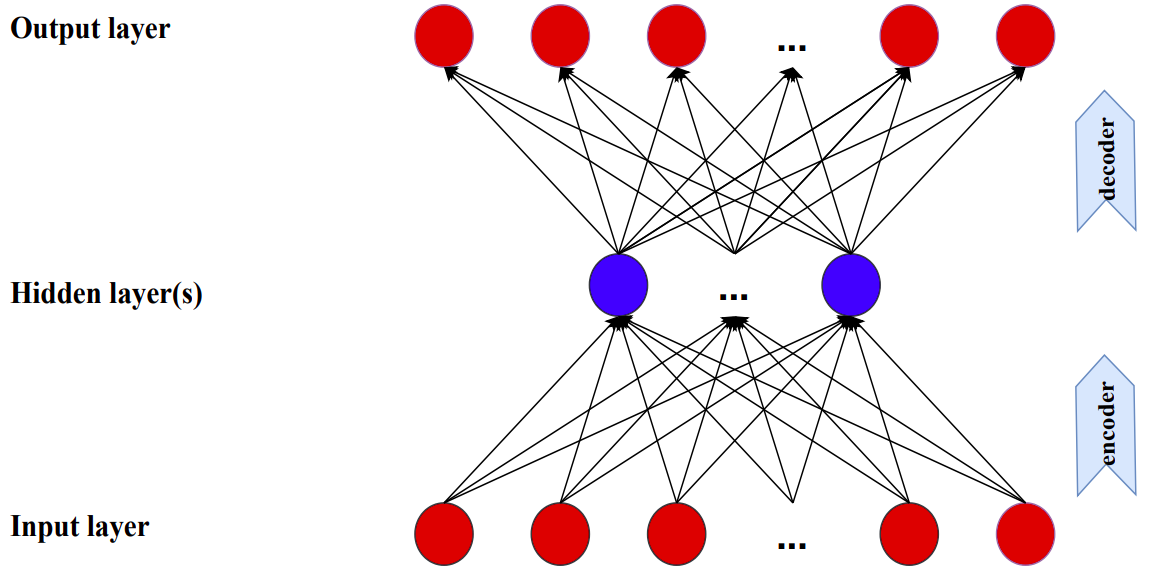
Autoencoders
- Neural network for dimension reduction
- Output layer is the same as input layer
- Hidden layer(s) have fewer neurons
New Model
Conditional Autoencoder
- Covariates improve estimates of factor loadings and latent factors
- Design new neural network structure by augmenting a standard autoencoder to incorporate covariates
- \(r_{i,t}=\beta'_{i,t-1}f_t+u_{i,t}\)
Conditional Autoencoder
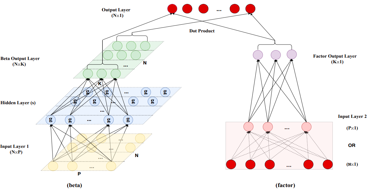
Beta (left side)
- Neural network to compute betas:
z^{(0)}_{i,t-1} = z_{i,t-1} \\
z^{(l)}_{i,t-1} = g\left(b^{(l-1)}+W^{(l-1)}z^{(l-1)}_{i,t-1}\right),\quad l-1,\dots,L_\beta \\
\beta_{i,t-1}=b^{(L_\beta)}+W^{(L_\beta)}z^{(L_\beta)}_{i,t-1}
Factor (right side)
- Neural network to compute betas:
r^{(0)}_{t} = r_t \\
r^{(l)}_t = \widetilde g\left(\widetilde b^{(l-1)}+\widetilde W^{(l-1)}r^{(l-1)}_t\right),\quad l-1,\dots,L_f \\
f_t=\widetilde b^{(L_f)}+\widetilde W^{(L_f)}r_t^{(L_f)}
- \(L_f=1\)
- This makes the factors interpretable as portfolios
Factor (right side)
- Difficult to use full cross section of individual stock returns
- Many weight parameters: 30,000 firms, 720 months
- Panel is unbalanced: only 6,000 stocks/month
- Solution: initialize network with set of portfolios
- \(x_t=(Z'_{t-1}Z_{t-1})^{-1}Z_{t-1}r_t\)
- Set of portfolios dynamically re-weighted by characteristic
- \(j^{th}\) element: return of long-short portfolio constructed by sorting stocks based on \(j^{th}\) characteristic
Objetive Function
- \(\theta\): summarizes weight parameters
- \(\phi(\theta)\): penalty function for regularization
- Use LASSO (\(l_1\))
- \(\phi(\theta;\lambda)=\lambda \sum_j |\theta_j|\)
- Set coefficients on a subset of covariates to exactly zero
- Imposes sparsity on weights
\mathcal L(\theta;\cdot) = \frac{1}{NT}\sum_{t=1}^T\sum_{i=1}^N ||r_{i,t}-\beta'_{i,t-1}f_t||^2+\phi(\theta;\cdot)
Other Regularization Techniques
- Early stopping: stop when validation sample errors begin to increase
- Usually occurs before errors minimized in training
- Ensemble: train 10 networks and use average prediction
Optimization Algorithn
- Stochastic gradient descent
- Adam optimizer
- Batch normalized: for each hidden layer in each training step (batch), cross-sectionally de-mean and standardize
- Motivated by internal covariate shift: inputs of hidden layers follow different distributions than their counterparts in the validation sample
- Should restore representation power of the unit
Data
Dataset
- Source: CRSP monthly data from NYSE, AMEX, and NASDAQ
- Range: March 1957 to December 2016 (60 years)
- 30,000 total stocks, ~6,200 per month
- Training: 1957-1974 (18 years)
- Validation: 1975-1986 (12 years)
- Testing: 1987-2016 (30 years)
Characteristics
- 94 characteristics
- 61 updated annually
- 13 updated quarterly
- 20 updated monthly
- Delay characteristics to avoid forward looking bias:
- Monthly by 1 month
- Quarterly by 4 months
- Annually by 6 months
- Avoid recursively refitting model each month
- Refit annually (most signals annual)
Characteristics
- Missing characteristics replaced by cross-sectional median of that characteristic for that month
- Distributions can be skewed and leptokurtic
- Rank-normalize characteristics
- Create 94 managed portfolios
- Also include one equal weighted market portfolio
- No filters based on prices or share types
Experiment
Model Set
- PCA: linear, constant betas, no conditioning
- IPCA: linear, conditional betas
- CA0: conditional autoencoder, single layer in both beta and factor networks (similar to IPCA)
- CA1: add hidden layer with 32 neurons to beta
- CA2: add second hidden layer with 16 neurons to beta
- CA3: add third hidden layer with 8 neurons to beta
- FF: Fama-French model with observable factors
- Try each model with 1 to 6 factors
Metrics
R^2_{total} = 1-\frac{\sum_{(i,t)\in OOS} (r_{i,t}-\hat\beta'_{i,t-1}\hat f_{t})^2}{\sum_{(i,t)\in OOS}r^2_{i,t}}
R^2_{pred} = 1-\frac{\sum_{(i,t)\in OOS} (r_{i,t}-\hat\beta'_{i,t-1}\hat \lambda_{t-1})^2}{\sum_{(i,t)\in OOS}r^2_{i,t}}
- \(\hat\lambda_{t-1}\): sample average of \(\hat f\) up to month \(t-1\)
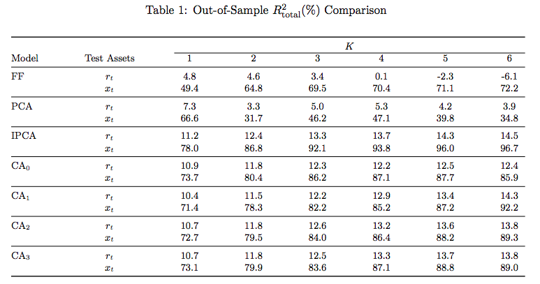
Results
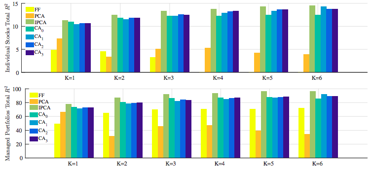
OOS \(R^2_{total}\)
- IPCA with 6 factors top performing
- Closely followed by CA networks
- FF models worst:
- Infrequent re-estimation of parameters
- Much larger cross-section of stocks than normal
OOS \(R^2_{total}\)
OOS \(R^2_{total}\)
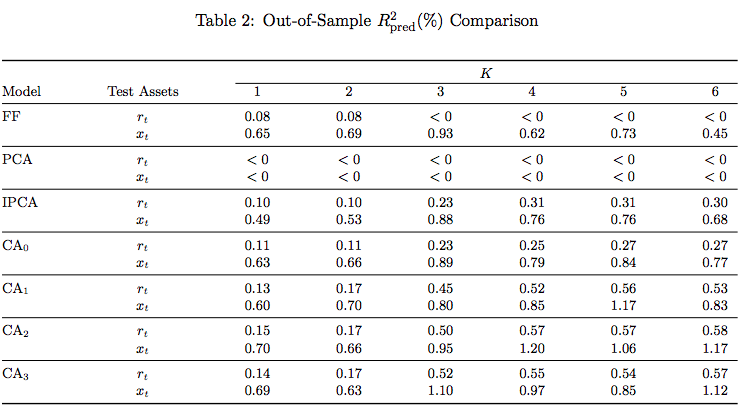
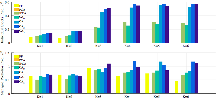
OOS \(R^2_{pred}\)
- CAs did much better than IPCA
- Static models did poorly
OOS \(R^2_{pred}\)
OOS \(R^2_{pred}\)
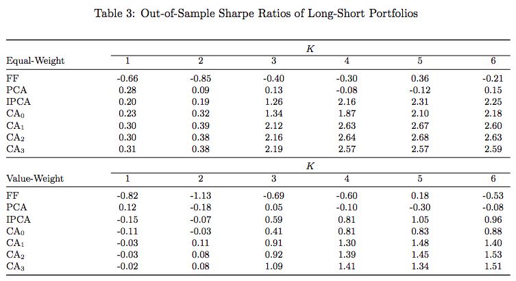
Economic Performance
- Sort stocks based on OOS forecast
- Create zero-net investment portfolio
- Buy top 10%
- Sell bottom 10%
- Equal-weighted and value-weighted portfolios
- CA2 top performing
Economic Performance
Economic Performance
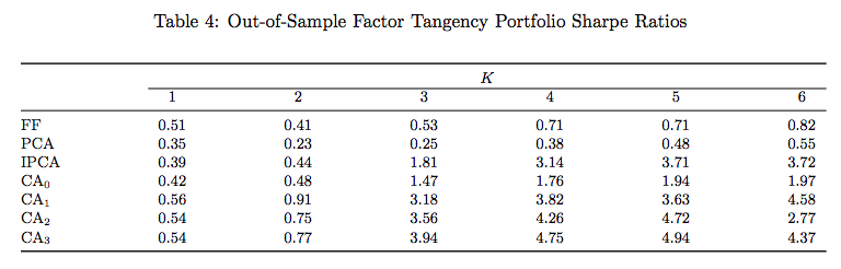
- Constructed using mean and covariance matrix of estimated factors through \(t\) and tracking the post-formation \(t+1\) return
- CA3 5-factor top performing
- Not necessarily implementable strategies
Risk Premia vs. Mispricing
- Models above specified with no intercept (\(\alpha\))
- Imposes no arbitrage
- Stock characteristics proxy for compensated factor risk exposures
- Should there be an intercept?
Risk Premia vs. Mispricing
- If zero-intercept is correct model, time series average of model residuals for each asset should be statistically indistinguishable from zero
- \(\alpha_i := E[u_{i,t}]=E[r_{i,t}]-E[\beta'_{i,t-1}f_t]\)
- Use \(t\)-tests

Risk Premia vs. Mispricing
- Magnitude of alphas less for CA
- Fewer are significant
- Those that are have small magnitude (7 bps/mo)
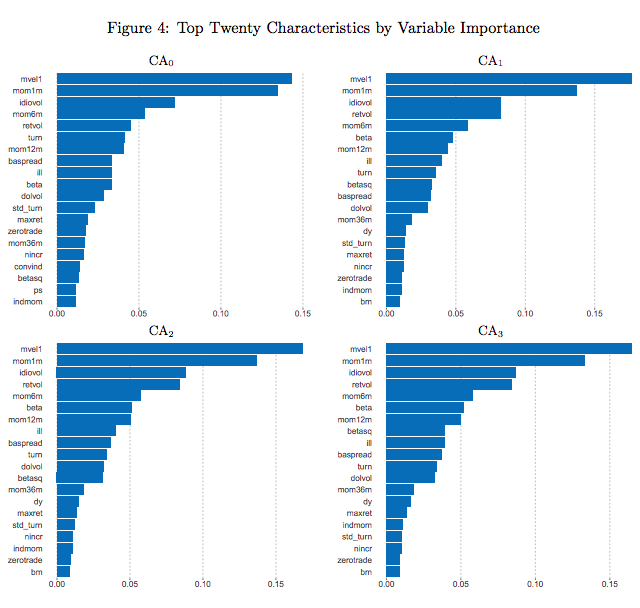
Characteristics Importance
- Variable importance by reduction in \(R^2_{total}\) when removed
- Top 20 characteristics contributed 90% for CA1-3
- Three influential categories:
- Price trend: reversal, momentum
- Liquidity: turnover, dollar volume, bid-ask spread
- Risk measures: volatility, market beta
Robustness Check
- Rerun on random subsamples
- Still performs well
Monte-Carlo Simulations
- Construct a dataset and test on it
- Performs well
Conclusion
- New nonlinear conditional asset pricing model
- Embeds economic restriction of no-arbitrage
- Dominates other asset pricing models
- Especially in predictive power
Analysis
- Well written and robust
- Like that they note perhaps not implementable
- Powerful framework for evaluating all characteristics
- Personally biased against monthly studies
- Need to look back far
- Market much different 50 years ago
- Their model can handle daily data/characteristics
- Would like to see study with short return periods and higher frequency characteristics
Autoencoder Asset Pricing Models
By Connor Chapin
Autoencoder Asset Pricing Models
Presentation on Autoencoder Asset Pricing Models