
Chad Scherrer
Senior Data Scientist, Metis
https://bit.ly/2SNDr1N
Follow Along Live
About Me
Served as Technical Lead for language evaluation for the DARPA program
Probabilistic Programming for Advancing Machine Learning (PPAML)
PPL Publications
-
Scherrer, Diatchki, Erkök, & Sottile, Passage : A Parallel Sampler Generator for Hierarchical Bayesian Modeling, NIPS 2012 Workshop on Probabilistic Programming
-
Scherrer, An Exponential Family Basis for Probabilistic Programming, POPL 2017 Workshop on Probabilistic Programming Semantics
- Westbrook, Scherrer, Collins, and Mertens, GraPPa: Spanning the Expressivity vs. Efficiency Continuum, POPL 2017 Workshop on Probabilistic Programming Semantics
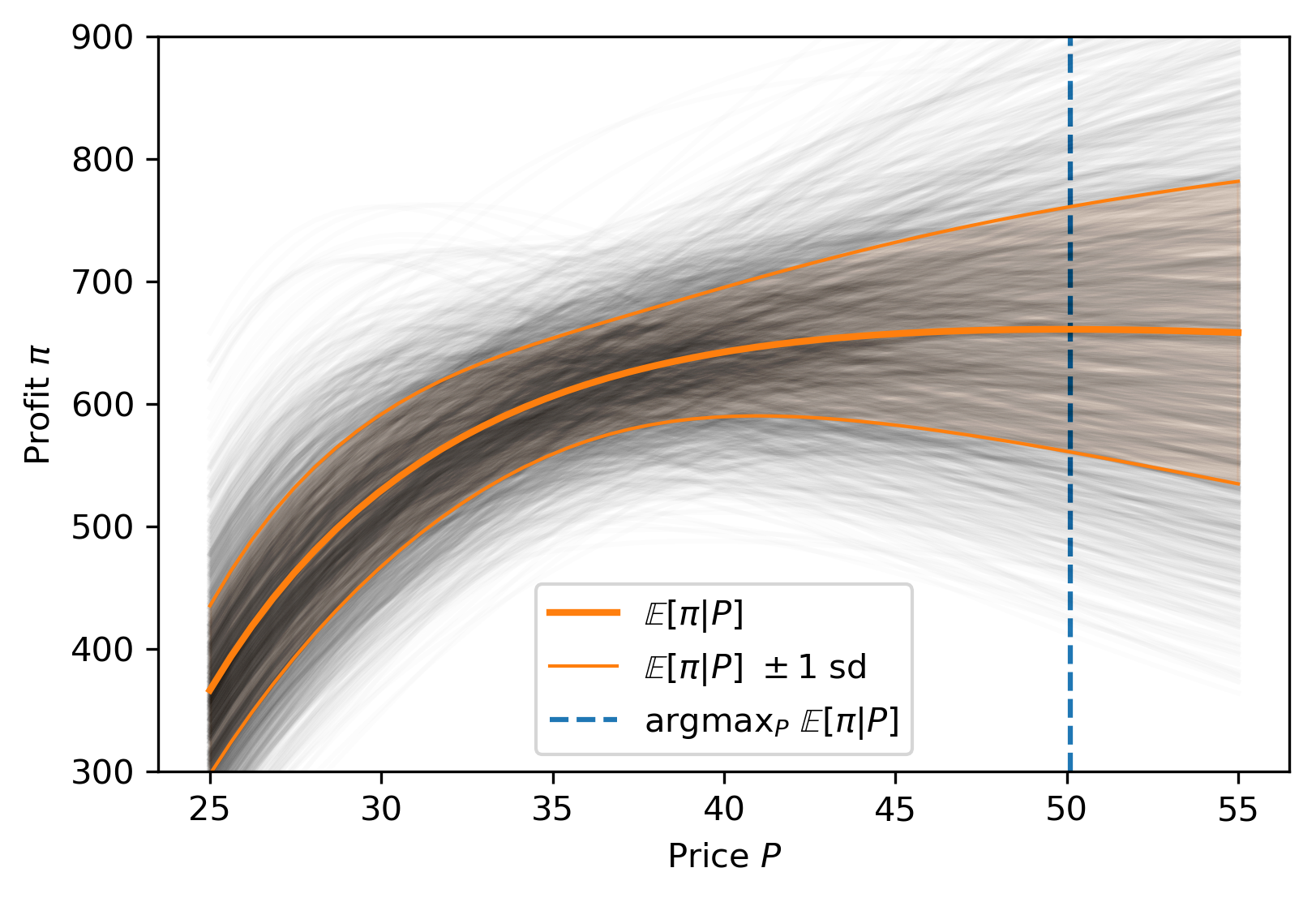
Making Rational Decisions
Managed Uncertainty
Rational Decisions
Bayesian Analysis
Probabilistic Programming
- Physical systems
- Hypothesis testing
- Modeling as simulation
- Medicine
- Finance
- Insurance
Risk
Custom models


Business Applications

Missing Data

The Two-Language Problem
A disconnect between the "user language" and "developer language"
X
3
Python
C
Deep Learning Framework
- Harder for beginner users
- Barrier to entry for developers
- Limits extensibility
?
A New Approach in Julia
- Models begin with "Tilde code" based on math notation
- A Model is a "lossless" data structure
-
Combinators transform code before compilation
Model
Tilde code
\begin{aligned}
\mu &\sim \text{Normal}(0,5)\\
\sigma &\sim \text{Cauchy}_+(0,3) \\
x_j &\sim \text{Normal}(\mu,\sigma)
\end{aligned}
μσxj∼Normal(0,5)∼Cauchy+(0,3)∼Normal(μ,σ)
Advantages
- Transparent
- Composable
- Backend-agnostic
- No intrinsic overhead
A Simple Example
P(\mu,\sigma|x)\propto P(\mu,\sigma)P(x|\mu,\sigma)
P(μ,σ∣x)∝P(μ,σ)P(x∣μ,σ)
\begin{aligned}
\mu &\sim \text{Normal}(0,5)\\
\sigma &\sim \text{Cauchy}_+(0,3) \\
x_j &\sim \text{Normal}(\mu,\sigma)
\end{aligned}
μσxj∼Normal(0,5)∼Cauchy+(0,3)∼Normal(μ,σ)
julia> nuts(m(:x), data=data, numSamples=10).samples
 (μ = 0.524, σ = 3.549)
 (μ = 3.540, σ = 2.089)
 (μ = 3.727, σ = 2.483)
 (μ = 3.463, σ = 2.582)
 (μ = 5.052, σ = 2.919)
 (μ = 4.813, σ = 1.818)
 (μ = 4.015, σ = 1.587)
 (μ = 5.244, σ = 3.949)
 (μ = 1.456, σ = 5.624)
 (μ = 4.045, σ = 2.010)
m = @model begin
    μ ~ Normal(0, 5)
    σ ~ HalfCauchy(3)
    x ~ Normal(μ, σ) |> iid
end
Theory
Soss.jl
Some Simple Model Combinators
m = @model begin
    μ ~ Normal(0, 5)
    σ ~ HalfCauchy(3)
    x ~ Normal(μ, σ) |> iid
end
julia> m(:x)
m = @model x begin
μ ~ Normal(0, 5)
σ ~ HalfCauchy(3)
x ~ Normal(μ, σ) |> iid
endjulia> m(x = [1.0, 1.1, 1.5])
@model begin
x = [1.0, 1.1, 1.5]
μ ~ Normal(0, 5)
σ ~ HalfCauchy(3)
x ~ Normal(μ, σ) |> iid
endObserve values statically
or dynamically
Composability: "First Class" Models
m1 = @model begin
    ...
end
mix = @model x,components begin
α = ones(length(components))
weights ~ Dirichlet(α)
x ~ MixtureModel(components,weights) |> iid
endjulia> mix(components=[m1, m2])
@model x begin
components = [m1, m2]
K = length(components)
weights ~ Dirichlet(ones(K))
x ~ MixtureModel(components, weights) |> iid
end
m2 = @model begin
    ...
end
Metaprogramming: Log-Density Calculation
function logdensity(model)
    body = postwalk(model.body) do x
        if @capture(x, v_ ~ dist_)
            assignment = ifelse(
                v ∈ parameters(model),
                :($v = par.$v),
                :($v = data.$v)
            )
            quote
                $assignment
                ℓ += logpdf($dist, $v)
            end
        else x
        end
    end

    return quote
        function(par, data)
            ℓ = 0.0
            $body
            return ℓ
        end
    end

end
julia> m(:x)
@model x begin
μ ~ Normal(0, 5)
σ ~ HalfCauchy(3)
x ~ Normal(μ, σ) |> iid
endjulia> logdensity(m(:x))
:(function (par, data)
ℓ = 0.0
μ = par.μ
ℓ += logpdf(Normal(0, 5), μ)
σ = par.σ
ℓ += logpdf(HalfCauchy(3), σ)
x = data.x
ℓ += logpdf(Normal(μ, σ) |> iid, x)
return ℓ
end)Static Dependency Analysis
julia> lda
@model (α, η, K, V, N) begin
    M = length(N)
    β ~ Dirichlet(repeat([η], V)) |> iid(K)
    θ ~ Dirichlet(repeat([α], K)) |> iid(M)
    z ~ For(1:M) do m
            Categorical(θ[m]) |> iid(N[m])
        end
    w ~ For(1:M) do m
            For(1:N[m]) do n
                Categorical(β[(z[m])[n]])
            end
        end
end
julia> dependencies(lda)
10-element Array{Pair{Array{Symbol,1},Symbol},1}:
[] => :α
[] => :η
[] => :K
[] => :V
[] => :N
[:N] => :M
[:η, :V, :K] => :β
[:α, :K, :M] => :θ
[:M, :θ, :N] => :z
[:M, :N, :β, :z] => :wBlei, Ng, & Jordan (2003). Latent Dirichlet Allocation. JMLR, 3(4–5), 993–1022.

Future Work
- More model types
- Online algorithms (Kalman filtering, etc)
- Model type hierarchy (StanLike <: Universal, etc)
- More back-ends
- Existing PPLs
- Variational inference (ADVI, Pyro-style, etc)
- More model combinators
- Non-centered parameterization
- Distributional approximation
- "Pre-Gibbs" decompositions

logo by James Fairbanks, on Julia Discourse site
JuliaCon 2019
July 21-27
Baltimore, MD
Thank You!

2019-01-11 PyData Miami
By Chad Scherrer
2019-01-11 PyData Miami
- 4,273


