ONLINE
MACHINE LEARNING
using Vowpal Wabbit
Darius Aliulis
About me
Software Engineer / R&D Scientist @ DATA DOG / SATALIA
Assistant lecturer @ Kaunas University of Technology
Business Big Data Analytics Master's study programme
Formal background in Applied Mathematics (MSc), studied
@ Kaunas University of Technology (KTU)
@ Technical University of Denmark (DTU)
Fields of interest
- Operational Machine Learning
- Streaming Analytics
- Functional & Reactive Programming
This talk
- gentle introduction online learning with Vowpal Wabbit
- keeping math to bare minimum
- with a simple usage example
- and links to further resources
Batch vs Online Learning (1)
-
Offline learning (batch) learning treats the dataset as a static, and evaluates the full dataset to make make a model parameter update, that is - to make a step in model parameter space.
- Online learning only looks at a single data point at a time and after evaluating it, makes a small incremental update to the model built so far. Several passes over a dataset may be done to converge to a solution.
Batch vs Online Learning (2)
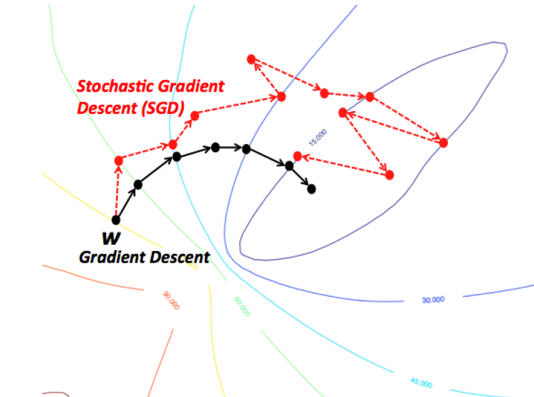
image source: https://wikidocs.net/3413
Intuition: Gradient Descent vs Stochastic Gradient Descent
Vowpal Wabbit (VW)
Fast out-of-core learning system started by John Langford, sponsored by Microsoft Research and (previously) Yahoo! Research
Used by multiple companies:
Yahoo, eHarmony, Nanigans, available as part Microsoft Azure ML, ...
A vehicle of advanced research - incorporates elements from over a dozen of papers since 2007.
Vowpal Wabbit (VW)
Vowpal Wabbit is also used for teaching the Master's course
P160M129 Multivariate Statistical Analysis Models
at Kaunas University of Technology for the \(3^{rd}\) year as an alternative tool to distributed processing for large scale machine learning.
Last but not least!
Vowpal Wabbit (VW)
Swiss army knife of online algorithms
Sharat Chikkerur, Principal data scientist lead @ Microsoft
- Linear Regression
- Quantile Regression
- Binary classification
- Multiclass classification
- Topic modelling (online Latent Dirichlet Allocation)
- Structured Prediction
- Active learning
- Recommendation (Matrix factorization)
- Contextual bandit learning (explore/exploit algorithms)
- Reductions
notable VW features
- Blazingly fast due to online learning
-
Flexible input format: multiple labels, numerical & categorical features
- No limit on dataset size due to streaming support
- No limit on feature space size due to hashing trick
- Distributed training with AllReduce
- Supports both online and batch optimization algorithms
VW setup
Ubuntu:
apt-get install vowpal-wabbitArch Linux: available on Archlinux User Repository (AUR)
Mac OS X:
brew install vowpal-wabbitCompile from source
OR
Links to precompiled binaries for Linux and Windows available on Download section of Github Wiki
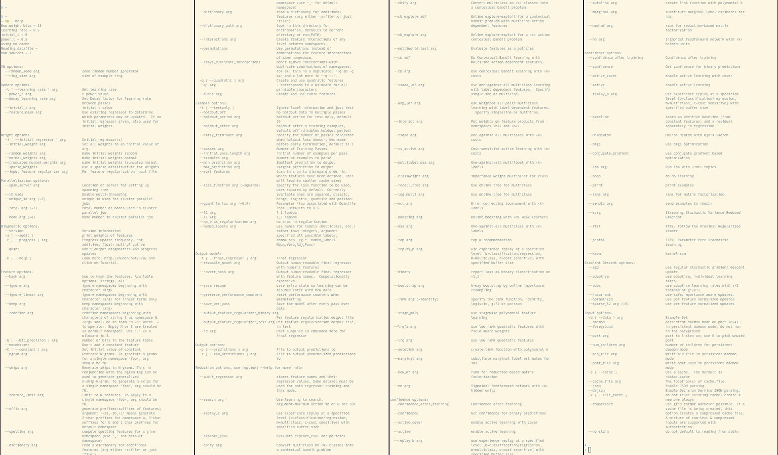
CLI - main VW interface*

*although wrappers (Python, Java) also available
Notes on VW feature hashing
Uses murmum hash v3 since August 2012.
Uses 32-bit version of the murmur v3 hash, so max \(2^{32} \approx 4\space \text{billion}\) features even on 64-bit machines.
The hash table, by default, can hold \(2^{18}\) or \(262\space 144\) entries. This can be changed with option
-b [ --bit_precision ] arg number of bits in the feature tablevw input format
For example, the tsv line
0 2 0 1 287e684f 0a519c5c 02cf9876is represented by this line for classification problem in VW format
-1 |n 1:2 2:0 3:1 4__287e684f 5__0a519c5c 6__02cf9876see Input Format in Github Wiki
[Label] [Importance] [Base] [Tag]|(namespace feature)...
namespace = String[:value]
feature = String[:value]
value = String|Float
Below is the VW format specification with [] as optional elements, and (...)* as optional repeats:
VW mini example
λ ~/talks/pycon2018/data
» head -n2 y.txt
5429.2315
5082.6640

λ ~/talks/pycon2018/data
» head -n2 X.txt
6.6697 77.9595 28.7488 5.3315 18.9925 45.0629 -8.3036
6.9342 109.9140 74.2774 103.1446 1.5695 4.4233 -9.6564
 123.3871 40.3022 51.7409 75.1570 103.2410 27.5286 16.
9115 30.2444
10.4579 63.3384 21.0568 3.9748 21.5462 49.4205 12.0003
 32.6279 107.4346 49.9549 85.6434 6.8445 18.2359 7.205
4 101.2997 25.1887 29.8518 55.7982 88.9854 31.3737 18.
4522 -0.6437
example dataset with 22-dimensional dataset \(\mathbf{x}\) values
VW model training
to train a simple linear regression model
vw --normalized \
--data training.vw \
--final_regressor serialized.vw_model \
--loss_function squared
with options
--normalized                          use per feature normalized updates
-f [ --final_regressor ] arg          Final regressor
-d [ --data ] arg                     Example Set
--loss_function arg (=squared)        Specify the loss function to be used,
                                      uses squared by default. Currently
                                      available ones are squared, classic,
                                      hinge, logistic, quantile and poisson.
y_{i}=\beta_{0}1+\beta_{1}x_{i1}+\cdots +\beta_{p}x_{ip}+\varepsilon_{i}=\mathbf{x}_{i}^{\top }{\beta }+{\varepsilon}_{i},\qquad i=1,\ldots ,n
here
\(y\) - response variable, \(p\) - #features, \(n\) - #observations, \(\varepsilon_i\) - error for \(i^{th}\) observation
\(\mathbf{x}_i\) feature vector of \(i^{th}\) observation, \(\beta\) - weight vector
execute command
VW loss function squared
Here we the squared loss function to train the linear regression model
see Loss Functions in Github Wiki for all loss functions
\text{L}_{i} = \frac{1}{2}(y_i - \hat{y}_i)^2,\qquad i=1,\ldots ,n
here
\(y\) - ground truth for \(i^{th}\) observation,
\(\hat{y}\) - predicted value for \(i^{th}\) observation,
\(n\) - #observations
VW predictions (1)
to make predictions with the trained model on a new dataset
validation.vw
execute command
vw \
--data validation.vw \
--initial_regressor serialized.vw_model \
--testonly \
--predictions preds_validation.txt
with options
-d [ --data ] arg                     Example Set
-i [ --initial_regressor ] arg        Initial regressor(s)
-t [ --testonly ]                     Ignore label information and just test
-p [ --predictions ] arg              File to output predictions to
VW predictions (2)
λ ~/talks/pycon2018/data [P]
» cat validation.vw | \
cut -d " " -f 1 | \
paste -d " " preds_validation.txt - | \
tail -n5
3107.101807 3139.4970
3527.003662 3282.8034
4397.797852 4567.4292
6931.407715 7570.2633
5317.828125 5271.9570
Let's make a sanity check on ground truth vs predictions
VW metrics
λ ~/talks/pycon2018/data [P]
» cat validation.vw | \
cut -d " " -f 1 | \
paste -d " " preds_validation.txt - \
> y_yhat.txt

λ ~/talks/pycon2018/data [P]
» mpipe metrics-reg y_yhat.txt --has-r2
MSE,MAE,R2
370083.86,485.77,0.77
Let's compute some regression metrics (using custom tools)
VW parameter weights (1)
to obtain parameter weights \(\beta\) with names of features \(\mathbf{x}\), use the same dataset as for training and execute command
vw \
--data training.vw \
--initial_regressor serialized.vw_model \
--audit_regressor weights.txt
with options
-d [ --data ] arg                     Example Set
-i [ --initial_regressor ] arg        Initial regressor(s)
--audit_regressor arg                 stores feature names and their
                                      regressor values. Same dataset must be
                                      used for both regressor training and
                                      this mode.
VW parameter weights (2)
λ ~/talks/pycon2018/data
» cat weights.txt
n^1:121005:0.0435846
n^2:121006:33.9805
n^3:121007:0.0872157
n^4:121008:11.0019
n^5:121009:0.143333
n^6:121010:0.105194
n^7:121011:0.102565
n^8:121012:41.1167
n^9:121013:-0.0541902
n^10:121014:-5.67916
n^11:121015:0.1747
n^12:121016:0.289733
n^13:121017:-0.0526699
n^14:121018:0.224619
n^15:121019:0.0570403
n^16:121020:0.138103
n^17:121021:-0.175711
n^18:121022:48.0092
n^19:121023:-1.01503
n^20:121024:0.0692328
n^21:121025:-0.0184649
n^22:121026:0.0639344
Constant:116060:-134.755
Is that all there is to VW?
NOT EXACTLY
VW options
Regularization
image source: scikit-learn docs
R(w) := \frac{1}{2} \sum_{i=1}^{n} w_i^2
L2 norm:
R(w) := \sum_{i=1}^{n} |w_i|
L1 norm:
leads to shrinked coefficients
leads to sparse coefficients
R(w) := \frac{\rho}{2} \sum_{i=1}^{n} w_i^2 + (1-\rho) \sum_{i=1}^{n} |w_i|
Elastic Net:

VW hyper-parameter tuning
Multiple options available for hyper-parameter tuning
- manual grid search - user specifies possible values for each parameter
- vw-hypersearch utility - written in Perl, available since forever
- vw-hyperopt.py utility - written in Python, available since version 8.2
- ... other external packages
vw-hypersearch args
see Using vw hypersearch in Github Wiki
» vw-hypersearch --help
vw-hypersearch version [unknown] calling Getopt::Std::getopts (version 1.12 [paranoid]),
running under Perl version 5.26.1.

Usage: vw-hypersearch [-OPTIONS [-MORE_OPTIONS]] [--] [PROGRAM_ARG1 ...]

The following single-character options are accepted:
	With arguments: -c -t -e
	Boolean (without arguments): -v -b -L

Options may be merged together.  -- stops processing of options.
Space is not required between options and their arguments.
  [Now continuing due to backward compatibility and excessive paranoia.
   See 'perldoc Getopt::Std' about $Getopt::Std::STANDARD_HELP_VERSION.]
Too few arguments...
Usage: vw-hypersearch [options] <lower_bound> <upper_bound> [tolerance] vw-command...

    Options:
        -t <TS>     Use <TS> as test-set file + evaluate goodness on it
        -c <TC>     Use <TC> as test-cache file + evaluate goodness on it
                    (This implies '-t' except the test-cache <TC> will be used
                     instead of <TS>)
        -L          Use log-space for mid-point bisection
        -e <prog>   Use <prog> (external utility) to evaluate how good
                    the result is instead of vw's own 'average loss' line
                    The protocol is: <prog> simply prints a number (last
                    line numeric output is used) and the search attempts
                    to find argmin() for this output.  You may also pass
                    arguments to the plugin using: -e '<prog> <args...>'

    lower_bound     lower bound of the parameter search range
    upper_bound     upper bound of the parameter search range
    tolerance       termination condition for optimal parameter search
                    expressed as an improvement fraction of the range

    vw-command ...  a vw command to repeat in a loop until optimum
                    is found, where '%' is used as a placeholder
                    for the optimized parameter

    NOTE:
            -t ... for doing a line-search on a test-set is an
            argument to 'vw-hypersearch', not to 'vw'.  vw-command must
            represent the training-phase only.
much simpler than for vw
vw-hypersearch example (1)
see also vw-hyperopt.py among utils in Github repository
vw-hypersearch \
-t validation.vw \
-L \
-- 1e-5 3e-1 1e-5 \
vw \
-f hs_serialized.vw_model \
-d training.vw \
--normalized \
--readable_model hs_readable.txt \
--holdout_off \
--l1 %
vw-hypersearch example (2)
vw-hypersearch: -L: using log-space search
trying 0.00584807733596198 ................................... 371877 (best)
trying 0.000512989112088496 ................................... 370071 (best)
trying 0.000114000028424641 ................................... 370153
trying 0.00129960064808189 ................................... 370209
trying 0.000288806345652925 ................................... 533716
trying 0.000731658635897043 ................................... 370093
trying 0.000411914506408425 ................................... 370059 (best)
trying 0.000359672962513046 ................................... 608388
trying 0.000447928661922046 ................................... 658723
trying 0.000391119580207898 ................................... 370057 (best)
trying 0.000378795944563211 ................................... 370055 (best)
trying 0.000371374456694477 ................................... 370054 (best)
trying 0.000366860609589695 ................................... 370054 (best)
trying 0.00036409837292253 ................................... 370053 (best)
trying 0.000362401625751134 ................................... 370053 (best)
trying 0.00036135693421297 ................................... 370053 (best)
trying 0.000360712785648755 ................................... 370053 (best)
trying 0.000360315254196644 ................................... 370053 (best)
trying 0.000360069785332528 ................................... 608737
trying 0.000360467045961816 ................................... 609101
trying 0.000360221473687834 ................................... 370053 (best)
trying 0.000360163526350602 ................................... 370053
trying 0.00036025729177333 ................................... 370053 (best)
trying 0.000360279430348314 ................................... 370053
trying 0.000360243610061722 ................................... 370053
trying 0.000360261519759823 ................................... 370053
0.000360257	370053
output
vw-hypersearch weights
λ ~/talks/pycon2018/data [P]
» vw --data training.vw \
--initial_regressor hs_serialized.vw_model \
--audit_regressor hs_weights.txt


λ ~/talks/pycon2018/data [P]
» cat hs_weights.txt
n^2:121006:33.7252
n^4:121008:11.075
n^8:121012:40.5486
n^10:121014:-5.71781
n^12:121016:0.904364
n^18:121022:47.4645
n^19:121023:-0.958524
Constant:116060:-89.4825
Let's output weigths of model with L1 regularization
vw-hypersearch metrics
λ ~/talks/pycon2018/data [P]
» cat validation.vw | \
cut -d " " -f 1 | \
paste -d " " preds_hs_validation.txt - \
> hs_y_yhat.txt

λ ~/talks/pycon2018/data [P]
» mpipe metrics-reg hs_y_yhat.txt --has-r2
MSE,MAE,R2
370052.98,485.55,0.77
Let's output metrics of model with L1 regularization for validation.vw dataset
No decrease in metrics with a simpler model
VW and Python
Python wrappers are available for Vowpal Wabbit
- Vowpal Wabbit Python Wrapper - vowpalwabbit package in main Github repo
- sklearn_vw module in vowpalwabbit package
- gensim wrapper of Latent Dirichlet Allocation for topic modelling
- ... other third party wrappers
VW and Python
Or simply
import subprocessand operate on the commands. Also read Data Science at the Command Line and look into Python packages meant for the command line
Additional Resources
- Vowpal Wabbit wiki on Github
https://github.com/JohnLangford/vowpal_wabbit/wiki
- FastML blog post series about VW
http://fastml.com/blog/categories/vw/
- Kaggle Vowpal Wabbit Tutorial
https://www.kaggle.com/kashnitsky/vowpal-wabbit-tutorial-blazingly-fast-learning
- Awesome Vowpal Wabbit list on Vowpal Wabbit Github wiki
Online Learning using Vowpal-Wabbit
By Darius Aliulis
Online Learning using Vowpal-Wabbit
Talk on Online Machine Learning @ PyCon 2018