Data Science, and Machine Learning With Python
(Data Analytics (overlapping and interrelated field))
[Artificial Intelligence]
(Comprehensively, AI is a multidisciplinary field that combines the power of data science, machine learning, and computer science, including additional academic subjects such as mathematics and statistical skills.)
DISCLAIMER: The images, code snippets...etc presented in this presentation were collected, copied and borrowed from various internet sources, thanks for them & credit to the creators/owner
Agenda
- What is Data Analytics and Data Science?
- What They Can Do?
- Prerequisites & Skillset
- Why Python
- Statistical Techniques (case study)
- Data Analytics & Visualizations (case study)
- Machine Learning (case study)
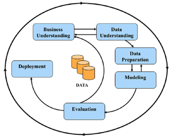
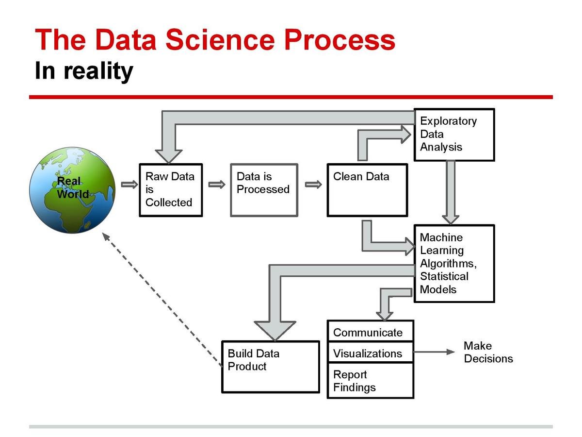
- D S & M L Project Workflow (End to End Project)
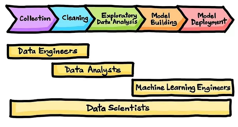
- Roles & Responsibilities
- Course Curriculum
- Q & A
What is Data Analytics?
Data Analytics is the process of inspecting, cleaning, transforming, and modeling data to discover useful information, draw conclusions, and support decision-making..
It transforms raw data into actionable insights, empowering businesses and professionals to make informed choices and drive strategic outcomes.
What is Data Science?
Data science is an interdisciplinary field. as it combines foundational ingredients from multiple disciplines and relevant domain knowledge to extract hidden patterns and trends or insights from data.
The ability to take data—to be able to understand it, to process it, to extract value from it, to visualize it, to communicate it—that’s going to be a hugely important skill in the next decades - Hal Varian
It encompasses various techniques and tools to analyze and interpret complex data sets.
The main goal of data science is to get valuable information and insights from the data that can be used to inform decision-making.
Data Science can be applied in many industries/sectors/fields such as healthcare, finance, marketing and retail, manufacturing, transportation, and many more.
What Data Analytics & Data Science Can Do?
-
Healthcare: Data science is used to analyze patient data and monitor vital signs in real-time to detect signs of illness or deterioration. This can be used to improve patient outcomes and reduce healthcare costs.
-
Finance: Data science is used in real-time to detect fraudulent transactions and monitor financial markets for signs of instability.
-
Retail and e-commerce: Data science is used to analyze customer data and track real-time sales trends to optimize inventory and pricing.
-
Transportation: Data science is used to analyze traffic and transportation data in real-time analyze customer data and track to optimize routes, reduce congestion, and improve traffic flow.
-
Manufacturing: Data science is used to monitor and analyze sensor data from manufacturing equipment to detect signs of wear and tear, optimize production processes, and improve efficiency.
-
Telecommunications: Data science is used to analyze network data in real-time to optimize performance, and detect and prevent service outages and fraud.
-
Agriculture: Data science is used to analyze sensor data from fields and weather patterns in real-time to optimize crop yields and reduce waste
this is actually just the tip of the iceberg
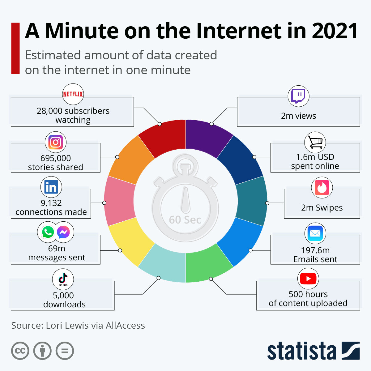
Data plays a huge part of modern life. And while data is revolutionising everything – from our shopping to our social lives – it is also transforming healthcare.
Why Python
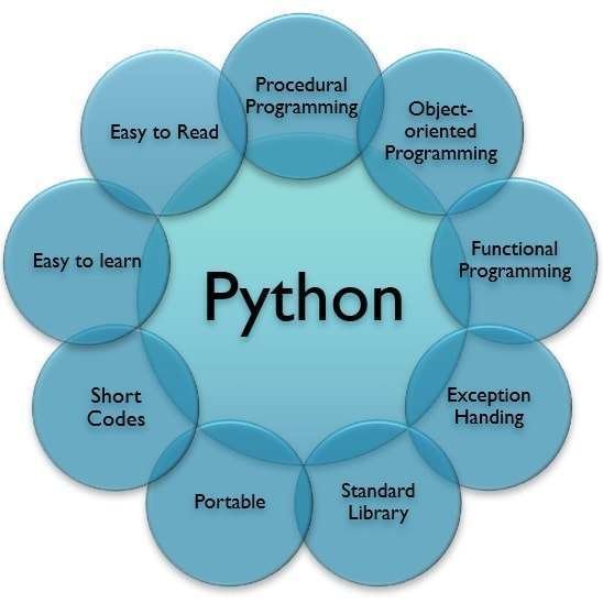
image source: https://bit.ly/3UVcgS6
Packages
- Numpy
- Pandas
- Matplotlib, Seaborn
- Sklearn
- .........etc
Statistics
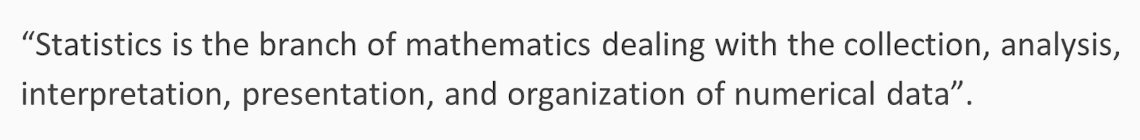
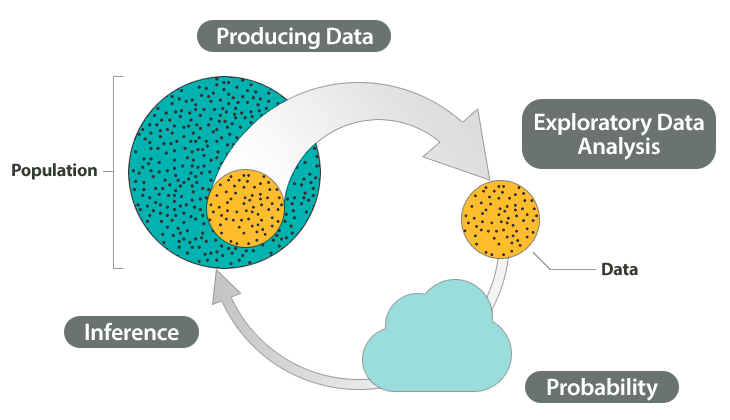
image source: https://bit.ly/3O5S26k
Elementary statistics
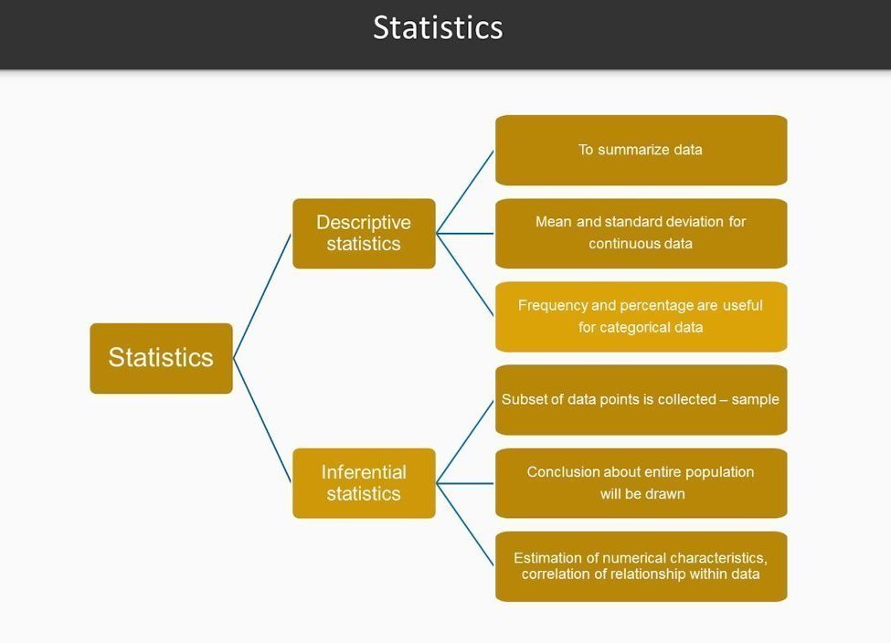
Statistics
Mean, Median, Mode, Standard Deviation, Range, Quartiles, skewness, kurtosis,.. more
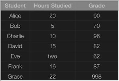
# Applying basic statistics in Python
import pandas as pd
data = {'Student': ['Alice',	'Bob',	'Charlie',	'David',	'Eve',	'Frank',	'Grace'],
        'Hours _Studied': [20,	5,	10,	15,	2,	16,	22],
        'Pre_Grade': [54,	78,	68,	67,	45,	57,	85],
        'Post_Grade': [90,	70,	96,	82,	62,	87,	98]}
df = pd.DataFrame(data, columns = ['Student', 'Hours _Studied', 'Pre_Grade', 'Post_Grade'])
print(df)
# Minimum value of Pre_Grade
df['Pre_Grade'].min()

# Maximum value of Pre_Grade
df['Pre_Grade'].max()

# The sum of all the Hours _Studied
df['Hours _Studied'].sum()

# Mean Pre_Grade
df['Pre_Grade'].mean()

# Median value of Post_Grade
df['Post_Grade'].median()

#Sample variance of Post_Grade values
df['Post_Grade'].var()

#Sample standard deviation of Post_Grade values
df['Post_Grade'].std()

# Cumulative sum of Pre_Grade, moving from the rows from the top
df['Pre_Grade'].cumsum()

# Summary statistics on Post_Grade
df['Post_Grade'].describe()
 Save
SaveData Analytics & Visualization
Data Analytics & Visualizations
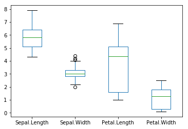
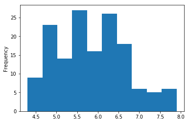
Summarize, Scatter plot, Histogram, Box plot, Pie chart, Bar plot, ...... more
# Basic plotting in Python

import pandas as pd
import matplotlib.pyplot as plt
iris = pd.read_csv("https://archive.ics.uci.edu/ml/machine-learning-databases/iris/iris.data",
                   header=None)
iris.columns = ['Sepal.Length', 'Sepal.Width', 'Petal.Length', 'Petal.Width',
       'Species']
iris.head()
iris['Sepal.Length'].plot(kind='hist')
iris.plot(kind='box')
plt.show()
iris.plot(kind='scatter', x='Sepal.Length', y='Sepal.Width')
plt.show()
Roles & Responsibilities
Machine Learning
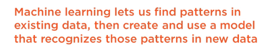
1. Start with a Question
3. Perform EDA
4. Apply Techniques
4. Share Insights
A Simple Example (DSML)
2. Get
& Clean the Data
1. Start with a Question
3. Perform EDA
4. Apply Techniques
5. Share Insights
if i study more, will i get a higher grade
2. Get
& Clean the Data
1. Start with a Question
3. Perform EDA
4. Apply Techniques
5. Share Insights
if i study more, will i get a higher grade
2. Get
& Clean the Data
1. Start with a Question
2. Get
3. Perform EDA
4. Apply Techniques
5. Share Insights
if i study more, will i get a higher grade
& Clean the Data
1. Start with a Question
3. Perform EDA
4. Apply Techniques
5. Share Insights
if i study more, will i get a higher grade
2. Get
& Clean the Data
1. Start with a Question
3. Perform EDA
4. Apply Techniques
5. Share Insights
if i study more, will i get a higher grade
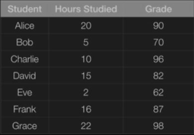
Finding #1: the more you study, the higher grade you will get
Finding #2: Also, Charlie is a smarty pants
2. Get
& Clean the Data
1. Start with a Question
3. Perform EDA
4. Apply Techniques
5. Share Insights
if i study more, will i get a higher grade
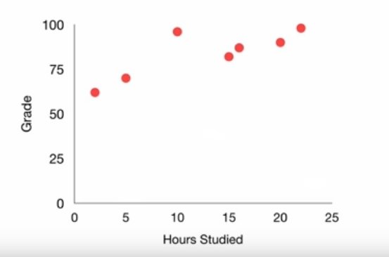
linear regression
Grade = 1.5*Hours + 65
2. Get
& Clean the Data
1. Start with a Question
3. Perform EDA
4. Apply Techniques
5. Share Insights
if i study more, will i get a higher grade
Yes, there is a positive correlation between the no of hours you study and the grade you get
Specifically, the relationship is Grade= 1.5*Hours + 65
So if you study 10 hrs, you can expect to get an 80
However, Charlie is a smarty pants and is inflating the grade estimate. You will probably get slightly less than 80
2. Get
& Clean the Data
import pandas as pd
from sklearn.linear_model import LinearRegression
from sklearn.model_selection import train_test_split
from sklearn.metrics import mean_squared_error, r2_score

# Load the dataset
df = pd.read_csv('student_data.csv')
df.dropna(subset=['grade'], inplace=True)

# Split the dataset into training and testing sets
X = df[['hours_studied']]
y = df['grade']
X_train, X_test, y_train, y_test = train_test_split(X, y, test_size=0.2, random_state=42)

# Create a Linear Regression model and fit the training data
model = LinearRegression()
model.fit(X_train, y_train)

# Make predictions on the testing set and calculate metrics
y_pred = model.predict(X_test)
mse = mean_squared_error(y_test, y_pred)
r2 = r2_score(y_test, y_pred)

print('Mean squared error:', mse)
print('R2 score:', r2)

# Make a prediction for a new student
new_hours_studied = [[6.5]] # hours studied for the new student
new_grade = model.predict(new_hours_studied)
print('Predicted grade:', new_grade)
Machine Learning Algorithm1
Local File
import pandas as pd
from sklearn.linear_model import LogisticRegression
from sklearn.model_selection import train_test_split
from sklearn.metrics import accuracy_score

# Load the Iris dataset into a Pandas dataframe
url = "https://archive.ics.uci.edu/ml/machine-learning-databases/iris/iris.data"
iris_data = pd.read_csv(url, names=["sepal_length", "sepal_width", "petal_length", "petal_width", "species"])

# Split the data into features (X) and labels (y)
X = iris_data[["sepal_length", "sepal_width", "petal_length", "petal_width"]]
y = iris_data["species"]

# Split the data into training and test sets
X_train, X_test, y_train, y_test = train_test_split(X, y, test_size=0.2, random_state=42)

# Create a logistic regression model
log_reg = LogisticRegression()

# Train the model on the training data
log_reg.fit(X_train, y_train)

# Use the model to make predictions on the test data
y_pred = log_reg.predict(X_test)

# Calculate the accuracy of the model
accuracy = accuracy_score(y_test, y_pred)
print("Accuracy:", accuracy)
Machine Learning Algorithm2
(Online Data)
# Generate Training Set
from random import randint
TRAIN_SET_LIMIT = 1000
TRAIN_SET_COUNT = 100

TRAIN_INPUT = list()
TRAIN_OUTPUT = list()
for i in range(TRAIN_SET_COUNT):
    a = randint(0, TRAIN_SET_LIMIT)
    b = randint(0, TRAIN_SET_LIMIT)
    c = randint(0, TRAIN_SET_LIMIT)
    op = a + (2*b) + (3*c)
    TRAIN_INPUT.append([a, b, c])
    TRAIN_OUTPUT.append(op)

# Train The Model
from sklearn.linear_model import LinearRegression

predictor = LinearRegression(n_jobs=-1)
predictor.fit(X=TRAIN_INPUT, y=TRAIN_OUTPUT)

# Test Data
X_TEST = [[10, 20, 30]]
outcome = predictor.predict(X=X_TEST)
coefficients = predictor.coef_

print('Outcome : {}\nCoefficients : {}'.format(outcome, coefficients))
Sample Machine Learning Model (with custom data)
from sklearn.model_selection import cross_val_score

# Create a logistic regression model
log_reg = LogisticRegression()

# Use cross-validation to estimate the model's performance
scores = cross_val_score(log_reg, X, y, cv=5)
print("Cross-validation scores:", scores)
print("Mean accuracy:", scores.mean())
Machine Learning Algorithm Complications and Handling Techniques
In real-world situations, it is unlikely that a model will achieve 100% accuracy. There are a few ways to make the above code less than 100% but better than average accuracy:
-
Use cross-validation: Its a technique that allows you to estimate the performance of a model on unseen data by dividing the data into multiple subsets, training the model on different subsets, and evaluating its performance on the remaining subsets. By using cross-validation, you can get a better estimate of the model's true performance.
Other Techniques such as Regularization, Feature scaling, Decreasing the sample size, or trying different algorithms and comparing the performance of each one, then choosing the one that performs better.
Here's an example of how you can modify the above code to use cross-validation to get an estimate of the model's true performance:
import matplotlib.pyplot as plt
import numpy as np
import pandas as pd
import sklearn.linear_model
# Load the data
oecd_bli = pd.read_csv("oecd_bli_2015.csv", thousands=',')
gdp_per_capita = pd.read_csv("gdp_per_capita.csv",thousands=',',delimiter='\t',
 encoding='latin1', na_values="n/a")
# Prepare the data
country_stats = prepare_country_stats(oecd_bli, gdp_per_capita)
"""
The prepare_country_stats() function’s definition is not shown here (see this chapter’s Jupyter notebook if
you want all the gory details). It’s just boring Pandas code that joins the life satisfaction data from the OECD
with the GDP per capita data from the IMF.
"""
def prepare_country_stats(oecd_bli, gdp_per_capita):
    oecd_bli = oecd_bli[oecd_bli["INEQUALITY"]=="TOT"]
    oecd_bli = oecd_bli.pivot(index="Country", columns="Indicator", values="Value")
    gdp_per_capita.rename(columns={"2015": "GDP per capita"}, inplace=True)
    gdp_per_capita.set_index("Country", inplace=True)
    full_country_stats = pd.merge(left=oecd_bli, right=gdp_per_capita,
                                  left_index=True, right_index=True)
    full_country_stats.sort_values(by="GDP per capita", inplace=True)
    remove_indices = [0, 1, 6, 8, 33, 34, 35]
    keep_indices = list(set(range(36)) - set(remove_indices))
    return full_country_stats[["GDP per capita", 'Life satisfaction']].iloc[keep_indices]

X = np.c_[country_stats["GDP per capita"]]
y = np.c_[country_stats["Life satisfaction"]]
# Visualize the data
country_stats.plot(kind='scatter', x="GDP per capita", y='Life satisfaction')
plt.show()
# Select a linear model
model = sklearn.linear_model.LinearRegression()
# Train the model
model.fit(X, y)
# Make a prediction for Cyprus
X_new = [[22587]] # Cyprus' GDP per capita
print(model.predict(X_new)) # outputs [[ 5.96242338]]
Decision tree
Random forest
K-Means
Naive Bayes
#Import Library
#Import other necessary libraries like pandas, numpy...
from sklearn import tree
#Assumed you have, X (predictor) and Y (target) for training data set and x_test(predictor) of test_dataset
# Create tree object
model = tree.DecisionTreeClassifier(criterion='gini') # for classification, here you can change the algorithm as gini or entropy (information gain) by default it is gini
# model = tree.DecisionTreeRegressor() for regression
# Train the model using the training sets and check score
model.fit(X, y)
model.score(X, y)
#Predict Output
predicted= model.predict(x_test)
#Import Library
from sklearn.ensemble import RandomForestClassifier
#Assumed you have, X (predictor) and Y (target) for training data set and x_test(predictor) of test_dataset
# Create Random Forest object
model= RandomForestClassifier()
# Train the model using the training sets and check score
model.fit(X, y)
#Predict Output
predicted= model.predict(x_test)
#Import Library
from sklearn.cluster import KMeans
#Assumed you have, X (attributes) for training data set and x_test(attributes) of test_dataset
# Create KNeighbors classifier object model
k_means = KMeans(n_clusters=3, random_state=0)
# Train the model using the training sets and check score
model.fit(X)
#Predict Output
predicted= model.predict(x_test)
#Import Library
from sklearn.naive_bayes import GaussianNB
#Assumed you have, X (predictor) and Y (target) for training data set and x_test(predictor) of test_dataset
# Create SVM classification object model = GaussianNB() # there is other distribution for multinomial classes like Bernoulli Naive Bayes, Refer link
# Train the model using the training sets and check score
model.fit(X, y)
#Predict Output
predicted= model.predict(x_test)
some important algorithms: https://goo.gl/zAyFea , https://bit.ly/2r59AWu
dataset = pd.read_csv('Social_Network_Ads.csv')
X = dataset.iloc[:, [2, 3]].values
y = dataset.iloc[:, 4].values
print(X)
print(y)

from sklearn.cross_validation import train_test_split
X_train, X_test, y_train, y_test = train_test_split(X, y, test_size = 0.25, random_state = 0)

from sklearn.preprocessing import StandardScaler
sc = StandardScaler()
X_train = sc.fit_transform(X_train)
X_test = sc.transform(X_test)

from sklearn.linear_model import LogisticRegression
classifier = LogisticRegression(random_state = 0)
classifier.fit(X_train, y_train

y_pred = classifier.predict(X_test)

from sklearn.metrics import confusion_matrix
cm = confusion_matrix(y_test, y_pred)
print(cm)

// import the function accuracy_score
from sklearn.metrics import accuracy_score

// prints the accuracy
print(accuracy_score(y_test, y_pred)*100)
Logistic Regression
# importing necessary libraries
from sklearn import datasets
from sklearn.metrics import confusion_matrix
from sklearn.model_selection import train_test_split

# loading the iris dataset
iris = datasets.load_iris()

# X -> features, y -> label
X = iris.data
y = iris.target

# dividing X, y into train and test data
X_train, X_test, y_train, y_test = train_test_split(X, y, random_state = 0)

# training a KNN classifier
from sklearn.neighbors import KNeighborsClassifier
knn = KNeighborsClassifier(n_neighbors = 7).fit(X_train, y_train)

# accuracy on X_test
accuracy = knn.score(X_test, y_test)
print (accuracy)

# creating a confusion matrix
knn_predictions = knn.predict(X_test)
cm = confusion_matrix(y_test, knn_predictions)
KNN classification
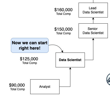
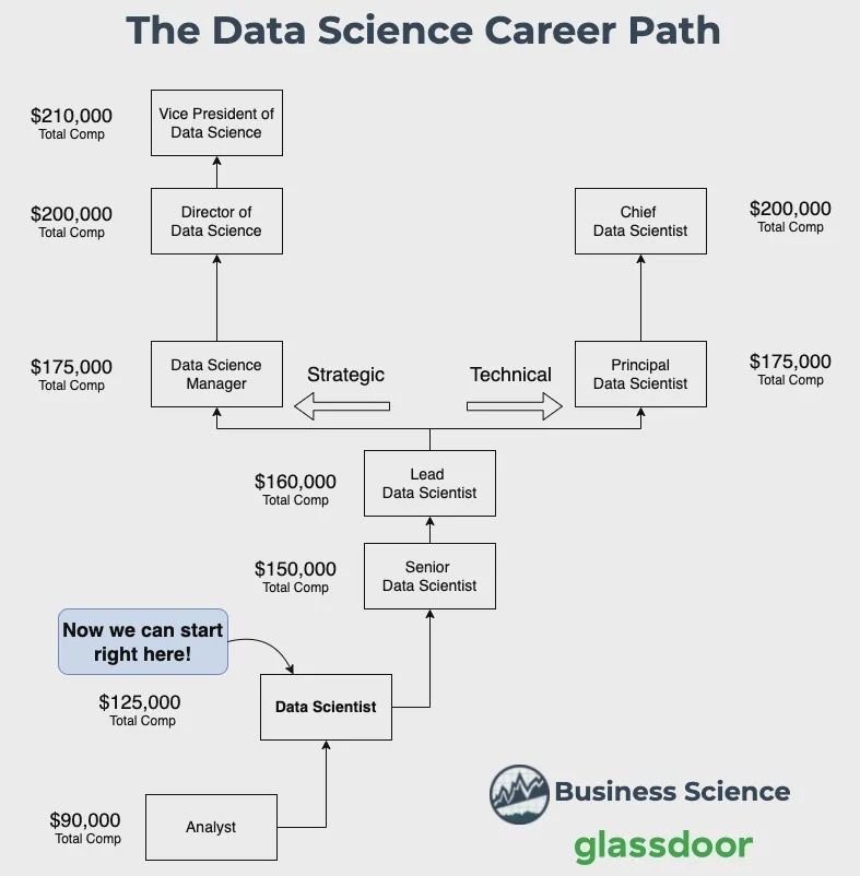
Data Science Skills are in High Demand Across Industries
Popular Programming Languages
TIOBE Index: https://www.tiobe.com/tiobe-index/
PYPL Ranking: https://pypl.github.io/PYPL.html
Top Programming Languages(IEEE Spectrum): https://bit.ly/3OMkbh6
(Linkedin, Glassdoor, Bureau of Labor Statistics & Payscale Reports)
Course Curriculum
Text
Final Note

Adjacent Tracks of DS AI ML Technology
-
Business Intelligence
-
Business Analytics
-
Big Data Analytics
-
Natural Language Processing (NLP)
-
ETL,ELT and Data Engineering
-
Deep Learning
-
Computer Vision
AI (Specialized Domains or Sub Tracks)
General Growth 1
Career Growth 2
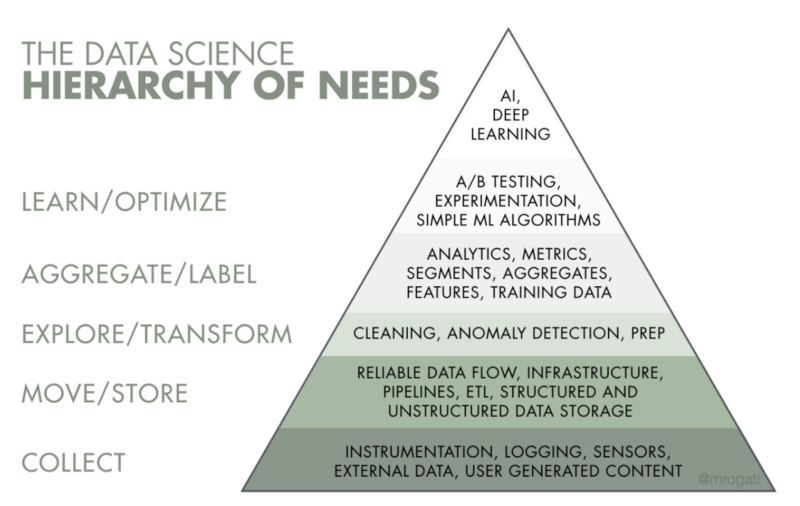
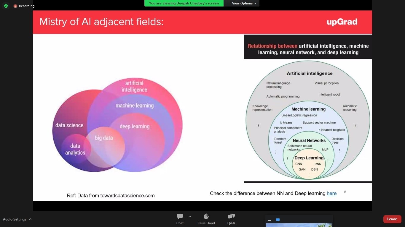
The AI Hierarchy
Top 10 Real-World Artificial Intelligence Applications: https://dzone.com/articles/ai-applications-top-10-real-world-artificial-intel
Skillsets
Skillsets
Natural Language Processing
Deep Learning
Demo & Practical (https://lobe.ai/)
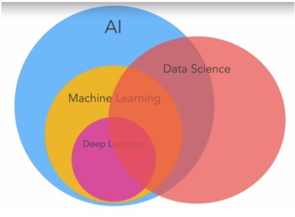
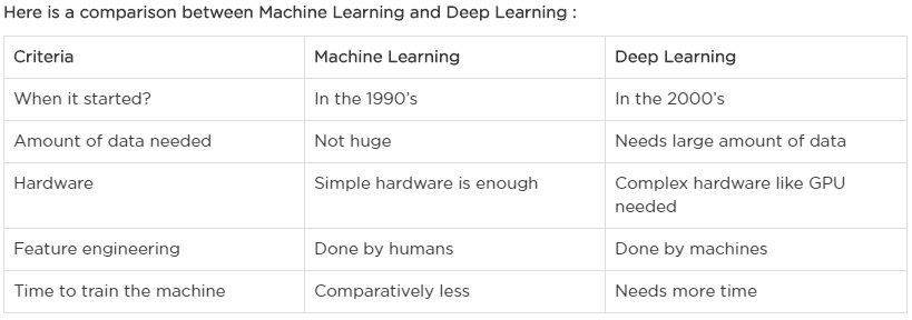
Machine Learning vs Deep Learning
Visual Understanding of Neural Network (DL) (https://jalammar.github.io/)
https://jalammar.github.io/visual-interactive-guide-basics-neural-networks/
https://jalammar.github.io/feedforward-neural-networks-visual-interactive/
https://github.com/jalammar/simpleTensorFlowClassificationExample/blob/master/Basic%20Classification%20Example%20with%20TensorFlow.ipynb
https://www.katacoda.com/basiafusinska/courses/tensorflow-getting-started/tensorflow-mnist-beginner
https://chromium.googlesource.com/external/github.com/tensorflow/tensorflow/+/r0.7/tensorflow/g3doc/tutorials/mnist/beginners/index.md
https://www.tensorflow.org/tutorials/quickstart/beginner
https://www.tensorflow.org/tutorials/keras/classification
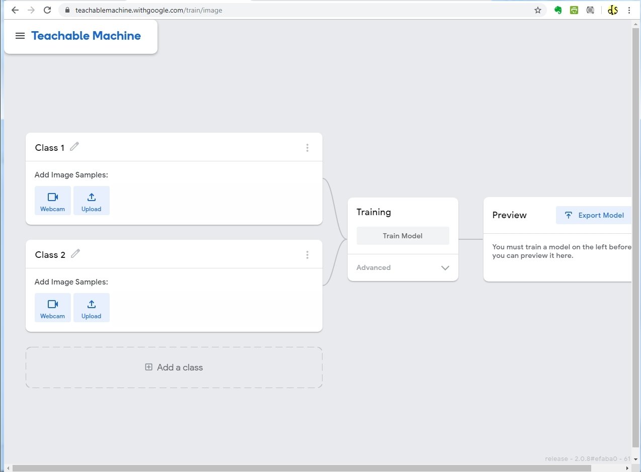
Deep Learning Demo & Practical (teachable machine)
MediaPipe Web-Enabled Machine Learning Framework: https://viz.mediapipe.dev/
The 12 Most Popular Computer Vision Tools in 2021:
https://viso.ai/computer-vision/the-most-popular-computer-vision-tools/
83 Most Popular Computer Vision Applications in 2022:
27+ Most Popular Computer Vision Applications and Use Cases in 2021:
Computer Vision
Difference between Deep Learning and Computer Vision
– Computer vision is a subset of machine learning that deals with making computers or machines understand human actions, behaviors, and languages similarly to humans. The idea is to get machines to understand and interpret the visual world so that they make sense out of it and derive some meaningful insights. Deep learning is a subset of AI that seeks to mimic the functioning of the human brain based on artificial neural networks.
Read more: Difference Between Computer Vision and Deep Learning | Difference Between http://www.differencebetween.net/technology/difference-between-computer-vision-and-deep-learning/#ixzz7HVNNNIJM
https://labs.openai.com/
https://platform.openai.com/playground
What is AI & 3 Types of AI (ANI,AGI,ASI):
https://codebots.com/artificial-intelligence/the-3-types-of-ai-is-the-third-even-possible
https://medium.com/mapping-out-2050/distinguishing-between-narrow-ai-general-ai-and-super-ai-a4bc44172e22
https://www.spiceworks.com/tech/artificial-intelligence/articles/narrow-general-super-ai-difference/
Copy of Data Science & Machine Learning with Python - demo
By Data Science Portal
Copy of Data Science & Machine Learning with Python - demo
Data Science & Machine Learning with Python


