A computational tool for neurodegenartive stratification using PET/RM


PI: Stefano De Marchi
RU participants:
Diego Cecchin (DIMED),
Maurizio Corbetta (DNS),
AnnaChiara Cagnin (DNS),
Cristina Campi (DIMA - UniGE).
PostDoc: Davide Poggiali (PNC)
Summary:
- Motivation: neurogenerative disease stratification.
- The sampling issue.
- "Fake Nodes" interpolation.
- 1D and 2D applications.
Neurodegenerative Disease Stratification
Data: an explorative dataset \(^{18}\)FdG-PET/MRI of ~150 subjects and counting (aged: 27-84) has been acquired, reconstructed, anonimized, stored in BIDS format.
Goal of the study: create an image-based tool to help the differential diagnosis in dementiae.
Six groups have been identified:
- Lewy-Body Dementia (DLB),
- Fronto-Temporal Dementia (FTD),
- Phenocopy of FTD (Pheno-FTD),
- Amyotrophic Lateral Sclerosis (ALS),
- Progressive Supranuclear Palsy (PSP),
- No sign of the above (N).
Neurodegenerative Disease Stratification
Template: to improve the segmentation accuracy an MRI template and a probability atlas were created using another set of MRIs from ~90 subjects (aged 30-95) affected by dementia.
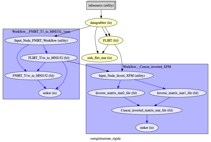
Pipeline: developed in nipype.
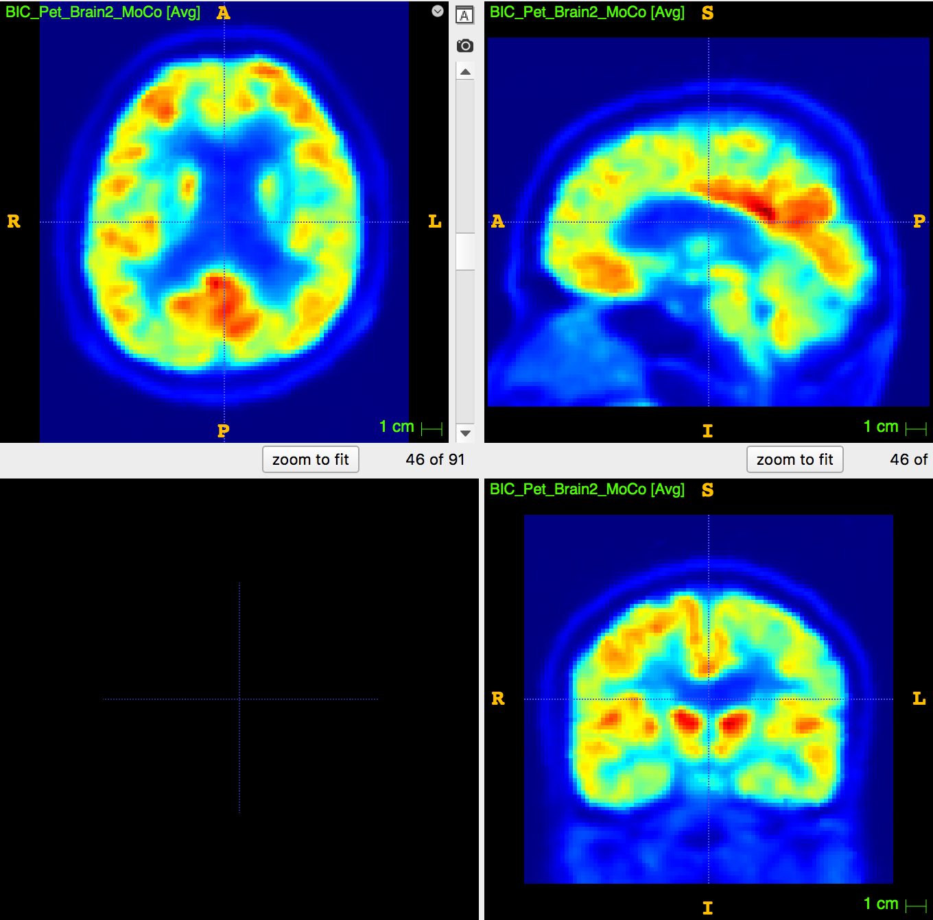
Neurodegenerative Disease Stratification
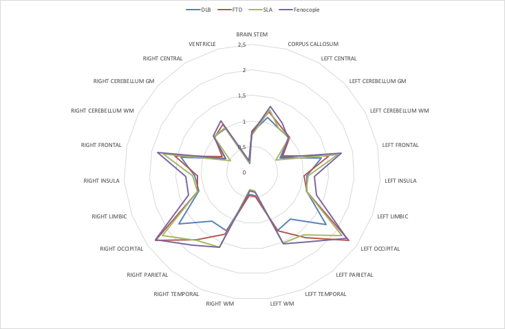
Mean PET-pvc, normalized by cerebellum GM, by lobule.
Explorative dataset results: (4 groups)
Neurodegenerative Disease Stratification
Confounding factors:
- Age/gender variability → normalization
- Inter-subject variability → unavoidable
- Resampling-derived errors → we will focus on the interpolation error and proposal of a workaround.
Stratification of patients is a difficult task.
- DLB is easy to identify
- FTD vs PhenoFTD difference is evident, but
- SLA vs FTD is not easy to distinguish from these data
Sampling problem in PET/MRI
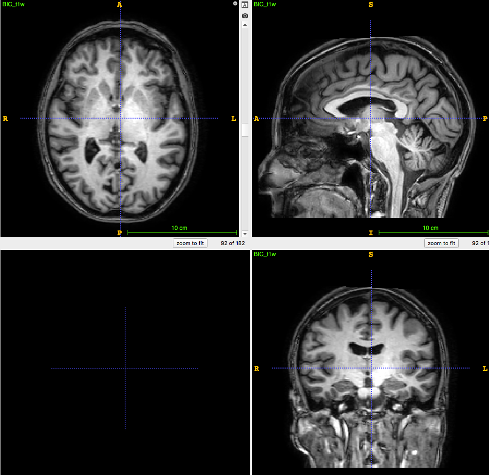
3D T1-weighted MRI:
usually ~1 mm \(^3\) voxel
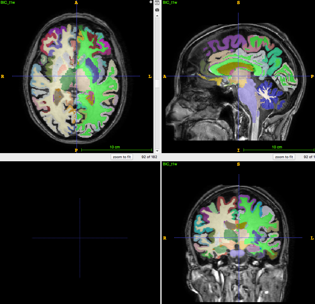
Segmentation/parcellation at full resolution
PET image:
usually ~8mm \(^3\) voxel
How to apply segmentation?
1. Undersampling T1 segmentation
2. Upsampling PET image
3. PET segmentation (no MRI)
Sampling problem in PET/MRI
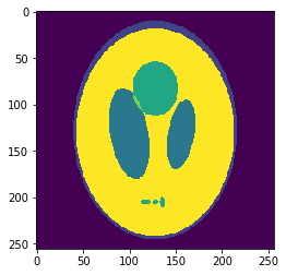
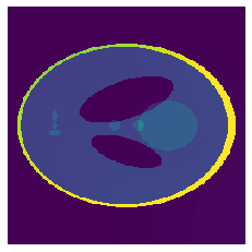
In silico test: Shepp-Logan 3D Phantom
Using a phantom the gold standard is known and we can analyse the errors of approximation.

High resolution "morphological" image
Segmentation mask
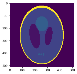
Low resolution "functional" image
Resampling is performed in ANTs
Original values at masks (gold standard):
g=[0.0, 1.0, 0.05, 0.3, 0.15, 0.2]
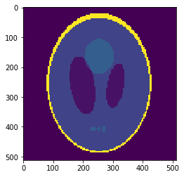
1mm^3
8mm^3
1mm^3
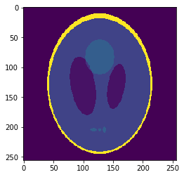
Downsampled segmentation mask
Low resolution "functional" image
Undersampling segmentation
The 2-norm relative error is \(\sqrt{\sum{ (g_i-v_i)^2 \over g_i^2}}\approx 0.058\)
Sampled mean values at masks:
v =[0.00033, 0.937, 0.0523, 0.298, 0.153, 0.206]
8mm^3
8mm^3
Oversampled "functional" image
Oversampling functional image
The 2-norm relative error is ~\(0.103\)
Segmentation mask
Sampled mean values at masks:
v=[0.0015, 0.889, 0.054, 0.297, 0.158, 0.209]
1mm^3
1mm^3
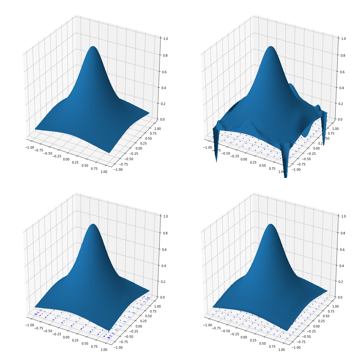
If we look at the pointwise interpolation error
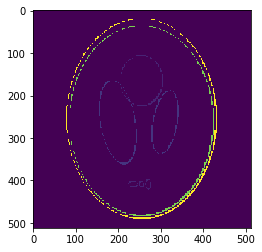
We can observe it is mostly higher distributed around the borders, where the gradient is higher.
This is what we call the
Gibbs phenomenon/effect.
Interpolation on "Fake Nodes", or interpolation via Mapped Bases is a technique in development by our group that applies to any interpolation method.
It has shown in many cases the ability of obtaining a
better interpolation without resampling!
This means that, it can be possible (in principle) to provide an interpolation of smaller error with a suitable mapping. "Fake nodes" interpolation has been tested as a solution to Runge and Gibbs phenomena with interesting results.
"Fake nodes" interpolation
Given a function
f: \Omega \subseteq \mathbb{R}^d \longrightarrow \mathbb{R}\;\;\;\;\; {d \in \mathbb{N}},
a set of nodes
X = \{ x_0, \dots, x_N \in \Omega \},
and a set of basis functions
\mathcal{B} = \{ b_i: \Omega \longrightarrow \mathbb{R} \}_{i = 0, \ldots, N}
The interpolant is given by a function
\displaystyle \mathcal{P}(\bm{x}) = \sum_{i=0}^{N} c_i b_i(\bm{x})
s.t.
\mathcal{P}(\bm{x}_i)=y_i:=f(\bm{x}_i) \;\;\forall i
\mathcal{B} = \{ b_i \circ S: \Omega \longrightarrow \mathbb{R}^d \}_{i = 0, \ldots, N}
\displaystyle \mathcal{R}^s(\bm{x}) = \sum_{i=0}^{N} c_i b_i(S(\bm{x}))
\mathcal{R}^s(\bm{x}_i)=y_i:=f(\bm{x}_i) \;\;\forall i
What is fake nodes interpolation?
This process can be seen equivalently as:
1. Interpolation over the mapped basis
\[\mathcal{B}^s = \{b_i \circ S \}_{i=0, \dots, N}.\]
2. Interpolation over the original basis \(\mathcal{B}\) of a function \(g: S(\Omega) \longrightarrow\mathbb{R}\)
at the fake nodes
\[S(X) = \{S(x_i) \}_{i=0, \dots, N}.\]
\(g\in C^s\) must satisfy \(g(S(x_i)) = f(x_i)\;\;\forall i\).
If \(\mathcal{P} \approx g \) on \(S(X)\) with the original basis,
then \(\mathcal{R}^s = \mathcal{P} \circ S \approx f \) on \(X\)
Application in 1D and 2D cases
Gibbs effect (1D)
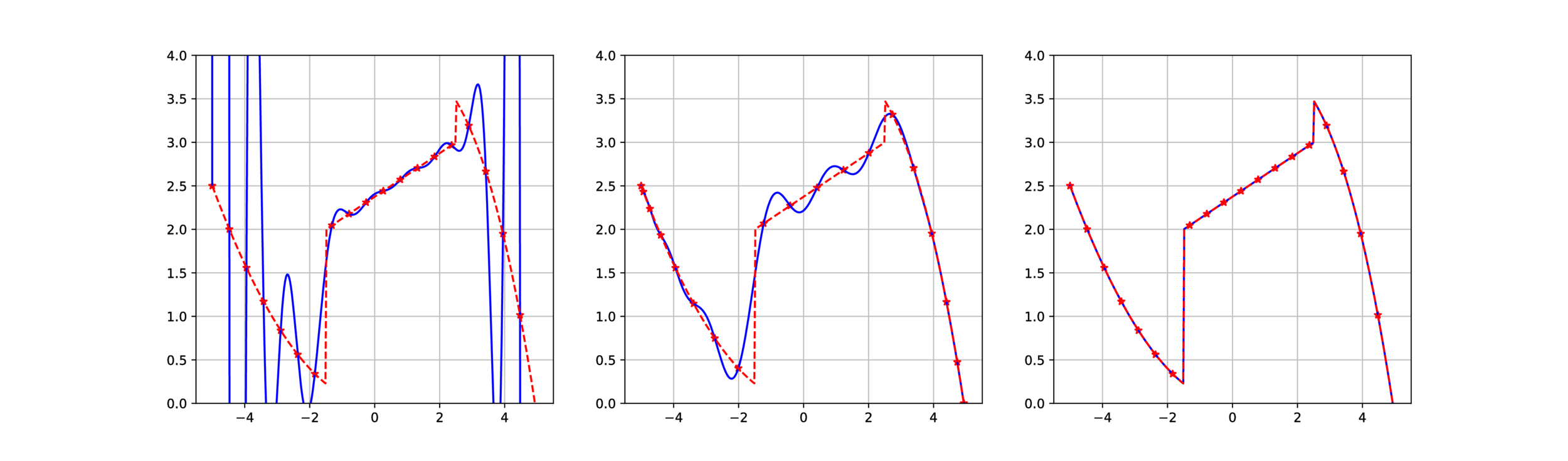
\displaystyle S(x) = x + \sum_{k=1}^m \alpha_k \chi_{\Gamma_k}(x)
\alpha_k \coloneqq k d_k
Application in 1D and 2D cases
Runge effect
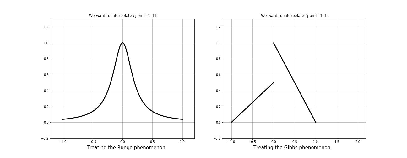
Gibbs effect
Application in 1D and 2D cases
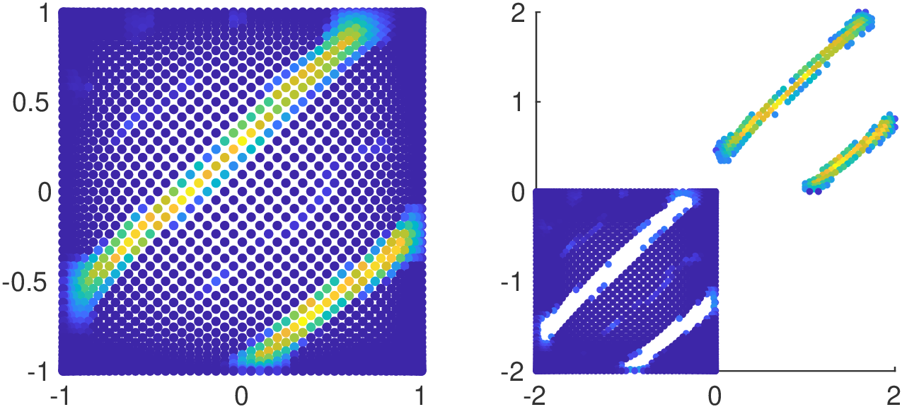
Gibbs effect (2D)
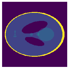
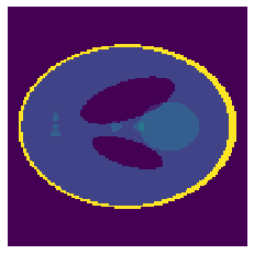
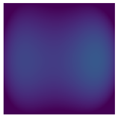
Original, high resolution image
Low resolution image
Polynomial upscaling (affected by Runge+Gibbs)
Fake Nodes upscaling
Application in 1D and 2D cases
Runge effect (2D)

Mapping to Chebyshev-Lobatto grid.
Mapping to Padua points.
Python code is available online https://github.com/pog87/FakeNodes
Application in 1D and 2D cases
Magnetic Particle Imaging (MPI)
Original nodes with corresponding values
Fake nodes with corresponding values
Application in 1D and 2D cases
Magnetic Particle Imaging (MPI)
Resampled results with RBF (Matern \(\mathcal{C}^0\))
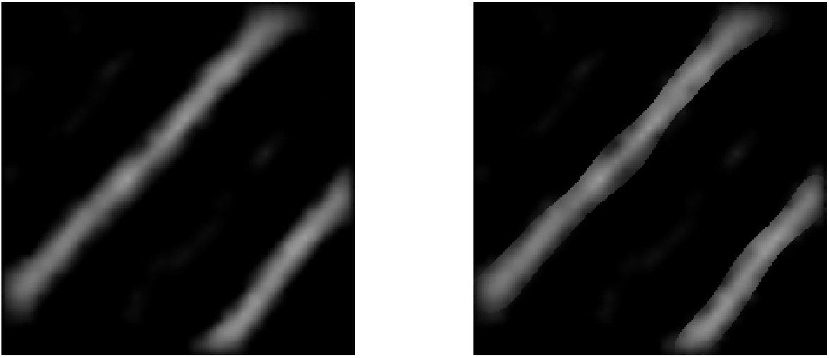
Resampled results with RBF (Matern \(\mathcal{C}^0\))
on Fake nodes
Next steps:
- Find a (possibly fast) Fake Nodes interpolation scheme in 3D,
- complete test on different phantoms,
- study the accuracy of the method on a physical PET phantom.
References
[1] B. Adcock, R.B. Platte, A mapped polynomial method for high-accuracy approximations on arbitrary grids, SIAM J. Numer. Anal, 2016.
[2J S. De Marchi, W. Erb, E. Francomano, F. Marchetti, E. Perracchione, D. Poggiali, Fake Nodes approximation for Magnetic Particle Imaging, Conference paper, MELECON 2020.
[3] S. De Marchi, F. Marchetti, E. Perracchione, Jumping with Variably Scaled Discontinuous Kernels (VSDKs), BIT Numerical Mathematics 2019.
[4] S. De Marchi, F. Marchetti, E. Perracchione, D. Poggiali, Polynomial interpolation via mapped bases without resampling, JCAM 2020.
[5] S. De Marchi, F. Marchetti, E. Perracchione, D. Poggiali, Multivariate approximation at Fake Nodes, AMC 2021.
[5] S. De Marchi, G. Elefante, E. Perracchione, D. Poggiali, Quadrature at Fake Nodes, preprint 2020.
[6] C. Runge, Uber empirische Funktionen und die Interpolation zwischen aquidistanten Ordinaten, Zeit. Math. Phys, 1901.
Thank you!
deck
By davide poggiali


