End-to-End Differentiable Simulations of Particle Accelerators
D. Vilsmeier
Artificial Neural Networks
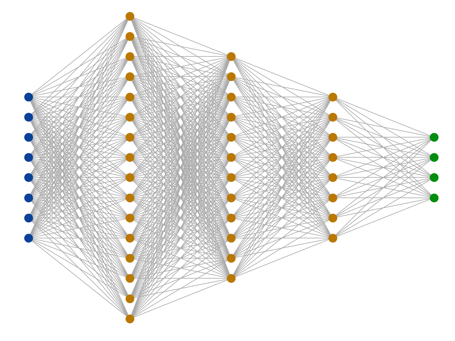
Example: "Fully connected, feed-forward network"
Input Layer
"Hidden" Layers
Output Layer
\vec{x}_n = \sigma\left(\bm{W}_n\cdot \vec{x}_{n-1} + \vec{b}_n\right)
Transformation per layer
Bias term
Weight matrix
(Non-)linear function ("activation")
\bm{W}_1
\vec{x}_0
\vec{x}_1
\vec{x}_2
\vec{x}_3
\vec{x}_4
\bm{W}_2
\bm{W}_3
\bm{W}_4
Input data
Prediction
- Used for mapping complex, non-explicit relationships
- E.g. image classification, translation, text / image / video generation, ...
- Data-driven algorithms
Optimization of network parameters
"Supervised Learning" using samples of input and expected output
Sample 🡒 Forward pass 🡒 Prediction
Quality of prediction by comparing with (expected) sample output, e.g. MSE
Minimization of loss by tuning network parameters 🡒 Optimization problem
Gradient based parameter updates using (analytically) exact gradients via Backpropagation algorithm
Dataflow &
Differentiable
Programming

Example: Particle Tracking
Example: Linear optics
x
p_x
y
p_y
t
p_t

x
p_x
y
p_y
t
p_t
M
Transfer Matrix
- Tracking through one element is analogue to a neural network layer (b = 0, σ = id)
- Weights are given and constrained by the transfer matrix
- Whole beamline is analogue to a feed-forward network
@ Entrance
@ Exit
Example: Particle Tracking
Example: Quadrupole
M = \begin{pmatrix}
\cos(\omega L) & \omega^{-1}\sin(\omega L) & 0 & 0 & 0 & 0 \\ \\
-\omega\sin(\omega L) & \cos(\omega L) & 0 & 0 & 0 & 0 \\ \\
0 & 0 & \cosh(\omega L) & \omega^{-1}\sinh(\omega L) & 0 & 0 \\ \\
0 & 0 & \omega\sinh(\omega L) & \cosh(\omega L) & 0 & 0 \\ \\
0 & 0 & 0 & 0 & 1 & \frac{L}{\beta_0^2\gamma_0^2} \\ \\
0 & 0 & 0 & 0 & 0 & 1
\end{pmatrix}
\omega = \sqrt{k_1} \; , \; k_1 = g / (B\rho)
x_1 = \cos(\sqrt{k}L)x_0 + \frac{\sin(\sqrt{k}L)}{\sqrt{k}}p_0
Tracking as computation graph
x_1 = \cos(\sqrt{k}L)x_0 + \frac{\sin(\sqrt{k}L)}{\sqrt{k}}p_0
Express as combination / chain of elementary operations
\textcolor{green}{x_1} = \textcolor{red}{\cos(}\color{red}\sqrt{\color{black}\textcolor{black}{k}}\textcolor{red}{\cdot} \textcolor{black}{L}\textcolor{red}{)}\textcolor{red}{\cdot} \textcolor{blue}{x_0} \textcolor{red}{+} \textcolor{red}{\sin(}\color{red}\sqrt{\color{black}\textcolor{black}{k}}\textcolor{red}{\cdot} \textcolor{black}{L}\textcolor{red}{)}\textcolor{red}{\cdot}\left(\color{red}\sqrt{\color{black}\textcolor{black}{k}}\right)^{\textcolor{red}{-1}}\textcolor{red}{\cdot}\textcolor{blue}{p_0}
Output / prediction
Input
(Elementary) operation
Parameter of element
Layout as computation graph (keeping track of operations and values at each stage)
Tracking as computation graph
k
\sqrt{}
\cdot^{-1}
\ast
\ast
L
\ast
\sin
\cos
\ast
+
p_0
x_0
x_1
\cos(\sqrt{\textcolor{orange}{k}}\cdot L)\cdot x_0 + \sin(\sqrt{\textcolor{orange}{k}}\cdot L)\cdot\left(\sqrt{\textcolor{orange}{k}}\right)^{-1}\cdot p_0
\cos(\textcolor{orange}{\sqrt{k}}\cdot L)\cdot x_0 + \sin(\textcolor{orange}{\sqrt{k}}\cdot L)\cdot\left(\textcolor{orange}{\sqrt{k}}\right)^{-1}\cdot p_0
\cos(\sqrt{k}\textcolor{orange}{\cdot L})\cdot x_0 + \sin(\sqrt{k}\textcolor{orange}{\cdot L})\cdot\left(\sqrt{k}\right)^{-1}\cdot p_0
\textcolor{orange}{\cos}(\sqrt{k}\cdot L)\cdot x_0 + \textcolor{orange}{\sin}(\sqrt{k}\cdot L)\cdot\left(\sqrt{k}\right)^{-1}\cdot p_0
\cos(\sqrt{k}\cdot L)\cdot x_0 + \sin(\sqrt{k}\cdot L)\cdot\color{orange}\left(\color{black}\sqrt{k}\color{orange}\right)^{\textcolor{orange}{-1}}\color{black}\cdot p_0
\cos(\sqrt{k}\cdot L)\textcolor{orange}{\cdot}\textcolor{blue}{x_0} + \sin(\sqrt{k}\cdot L)\cdot\left(\sqrt{k}\right)^{-1}\textcolor{orange}{\cdot}\textcolor{blue}{p_0}
\cos(\sqrt{k}\cdot L)\cdot x_0 + \sin(\sqrt{k}\cdot L)\textcolor{orange}{\cdot}\left(\sqrt{k}\right)^{-1}\cdot p_0
\cos(\sqrt{k}\cdot L)\cdot \textcolor{blue}{x_0} \textcolor{orange}{+} \sin(\sqrt{k}\cdot L)\cdot\left(\sqrt{k}\right)^{-1}\cdot \textcolor{blue}{p_0}
Tracking as computation graph
\cos(\sqrt{k}\cdot L)\cdot x_0 + \sin(\sqrt{k}\cdot L)\cdot\left(\sqrt{k}\right)^{-1}\cdot p_0
k
\sqrt{}
\cdot^{-1}
\ast
\ast
L
\ast
\sin
\cos
\ast
+
p_0
x_0
x_1
0.1
0.32
3.2
0.98
1.0
0.32
0.32
0.32
0.95
0.31
0.0295
0.0475
0.077
0.03
0.05
Tracking as computation graph
\cos(\sqrt{k}\cdot L)\cdot x_0 + \sin(\sqrt{k}\cdot L)\cdot\left(\sqrt{k}\right)^{-1}\cdot p_0
k
\sqrt{}
\cdot^{-1}
\ast
\ast
L
\ast
\sin
\cos
\ast
+
p_0
x_0
x_1
0.1
0.32
3.2
0.98
1.0
0.32
0.32
0.32
0.95
0.31
0.0295
0.0475
0.077
1.0
1
1.0
1.0
\textrm{r.h.s.}
\textrm{r.h.s.}
0.03
0.05
0.05
0.03
\textrm{r.h.s.}
0.096
0.009
-\sin
\cos
-0.016
0.091
\frac{d}{dk}x_1 \rightarrow \textrm{\small{chain rule}}
\textrm{r.h.s.}
0.075
-\left(\cdot\right)^{-2}
-0.091
\frac{1}{2\sqrt{}}
-0.025
Why not derive manually?

For long lattices this type of derivatives can become very quickly very tedious
Beamline consists of many elements
Tracking in circular accelerator requires multiple turns
Dependence on lattice parameters typically non-linear
Symbolic differentiation can help to "shortcut"
Example: Quadrupole tuning
- Beamline, 160 m, 21 quadrupoles, gradients are to be adjusted
- Fulfill multiple goals:
- Minimize losses along beamline
- Minimize beam spot size at target
- Keep beam spot size below threshold at beam dump location

21 Quadrupoles
Target
Beam dump
Envelope

Optimize gradients

Example: Inference of model errors
- Same beamline as before, infer quadrupole gradient errors w.r.t model
- Quality metric: mean squared error of simulated vs. measured Trajectory Response Matrix (TRM)
- TRM = orbit response @ BPMs in dependence on kicker strengths
\mathrm{TRM}_{\,mn}^{\,q = x,y} = \frac{q_{m,2} - q_{m,1}}{\theta_{n,2} - \theta_{n,1}}

beam position @ BPM
kicker strength
What about other optimizers?
Gradient-Free
Gradient-Approx.
Gradient-Exact
E.g. Nelder-Mead, Evolutionary algorithms, Particle Swarm, etc.
Any derivative-based method, e.g. via finite-difference approx.
Balance exploration vs. exploitation of the loss landscape (parameter space)
Exploration: Try out yet unknown locations
Exploitation: Use information about landscape to perform an optimal parameter update
No "built-in" exploration, but can be included via varying starting points (global) and learning rate schedules (local)
Symbolic differentiation or differentiable programming
Additional advantages
- Good convergence properties, also for (very) large parameter spaces
- No need to rely on plain vanilla gradient descent, all sort of advanced optimizers are available, e.g. RMSprop or Adam
- Two function evaluations per gradient computation (where e.g. finite-difference approx. uses N function evaluations)
- Running on GPU / TPU? Yes!
Deep learning packages provide straightforward ways to switch devices
→ "Batteries included"
https://commons.wikimedia.org/wiki/File:Geforce_fx5200gpu.jpg

Not limited to particle tracking nor linear optics
High versatility w.r.t. data and metrics

End-to-End Differentiable Simulations of Particle Accelerators
By Dominik Vilsmeier


