


18/09/2018
3rd IPM Workshop, D. Vilsmeier


Resolving Profile Distortion
for Electron-based IPMs
using Machine Learning
D. Vilsmeier (GSI)
M. Sapinski (GSI)
R. Singh (GSI)
3rd IPM Workshop
J-PARC (Tokai, Japan)
18/09/2018
3rd IPM Workshop, D. Vilsmeier
What is Machine Learning?
Field of study that gives computers the ability to learn without being explicitly programmed.
- Arthur Samuel (1959)


"Classical"
approach:
+
=
Input
Algorithm
Output
Machine
Learning:
+
=
Input
Algorithm
Output
18/09/2018
3rd IPM Workshop, D. Vilsmeier
Machine Learning Toolbox
Supervised Learning:
- Artificial Neural Networks
- Decision Trees
- Linear Regression
- k-Nearest Neighbor
- Support Vector Machines
- Random Forest
- ... and many more
Unsupervised Learning:
- k-Means Clustering
- Autoencoders
- Principal comp. analysis
Reinforcement Learning:
- Q-Learning
- Deep Deterministic Policy Gradient
18/09/2018
3rd IPM Workshop, D. Vilsmeier
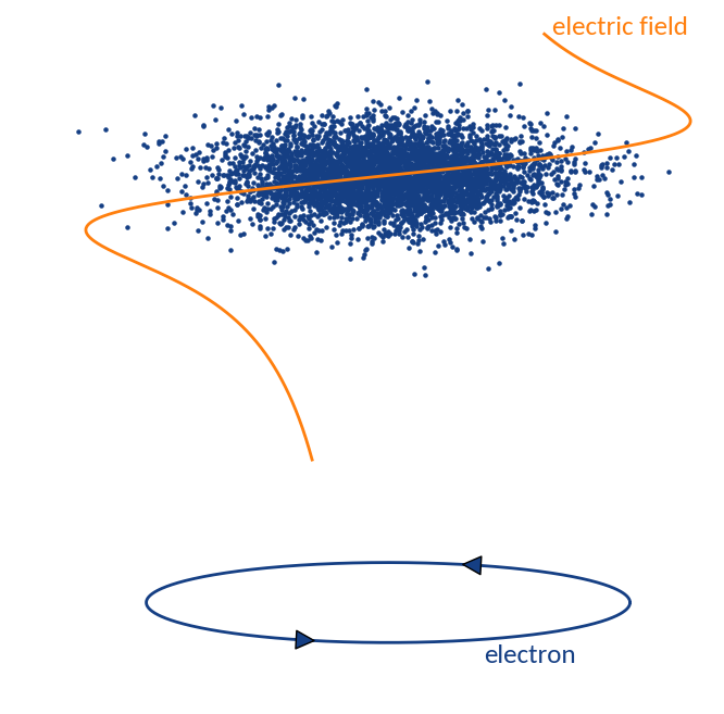
IPM Profile Distortion

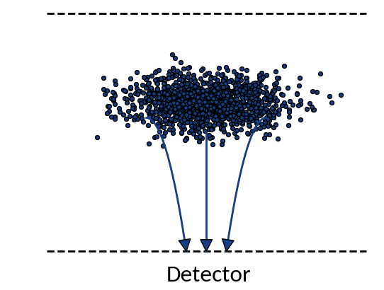
+V
-V
Ideal case
Particles move on straight lines towards the detector
Real case
Trajectories are influenced by initial momenta and by interaction with beam field
18/09/2018
3rd IPM Workshop, D. Vilsmeier
Counteract via ...
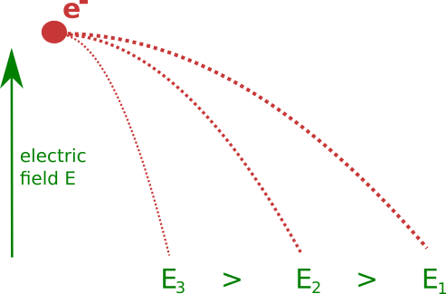
Increase of electric field
Resulting in smaller extraction times and hence smaller displacements; limit is quickly reached
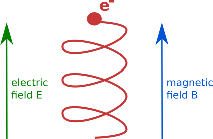
Additional magnetic field
Constrains the maximal displacement to the gyroradius of the resulting motion; usually an effective measure
18/09/2018
3rd IPM Workshop, D. Vilsmeier
Distortion without magnetic field
- Already observed in [W. DeLuca, IEEE 1969]
(+ observation of focusing for electron collection) -
R. E. Thern "Space-charge Distortion in the Brookhaven Ionization Profile Monitor" PAC 1987
- Simulations + Measurements
- Good agreement for nominal extraction voltages
- Disagreement at lower extraction voltages
- W. Graves "Measurement of Transverse Emittance in the Fermilab Booster" PhD 1994
\sigma_{\textrm{beam}} = c_1 + c_2\sigma_{\textrm{measured}} + c_3N
\sigma_m = \sigma + 0.302\frac{N^{1.065}}{\sigma^{2.065}}\left(1 + 3.6\,R^{1.54}\right)^{-0.435}
+ other approaches, including non-Gaussian beam shapes via iterative procedures
18/09/2018
3rd IPM Workshop, D. Vilsmeier
Distortion with magnetic field
- More complex motion also due to the interaction with beam electric field
- Capturing effects as well as different electromagnetic drifts play a role
-
Displacement from initial position can be mainly ascribed to three different effects:
- Displacement of gyro-center due to initial velocities
- Displacement of gyro-center due to space-charge interaction
- Displacement due to gyro-motion above detector
Space-charge region
Detector region

(\Delta x_1)
(\Delta x_2)
(\Delta x_3)
🠖 Final motion is determined by effects in the "space-charge region"
18/09/2018
3rd IPM Workshop, D. Vilsmeier
Electron trajectories
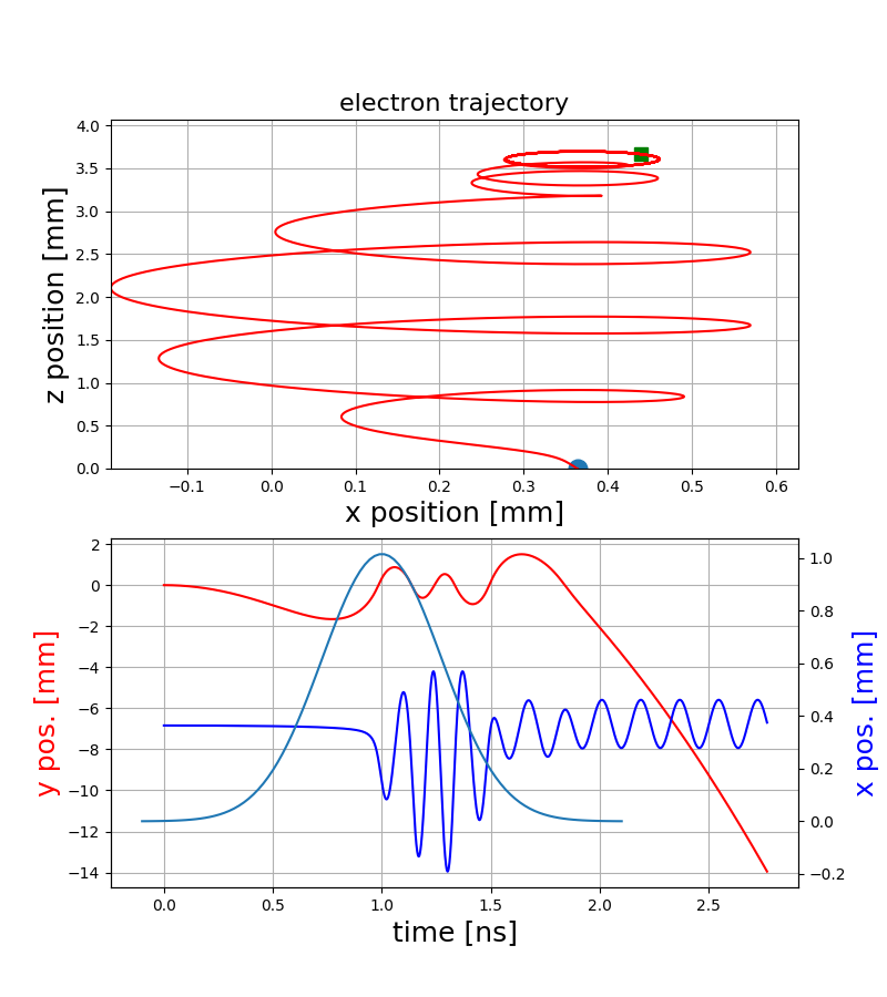
ExB-drift
Polarization drift
\left(\frac{d\vec{E}}{dt}\right)
Capturing
"Pure" gyro-motion
- The resulting motion strongly depends on the starting position within the bunch and hence on the bunch shape itself
- Various electromagnetic drifts / interactions create a complex dependence of the final gyro-motion on the initial conditions
p-bunch
Electron motion
18/09/2018
3rd IPM Workshop, D. Vilsmeier
Gyro-radius increase
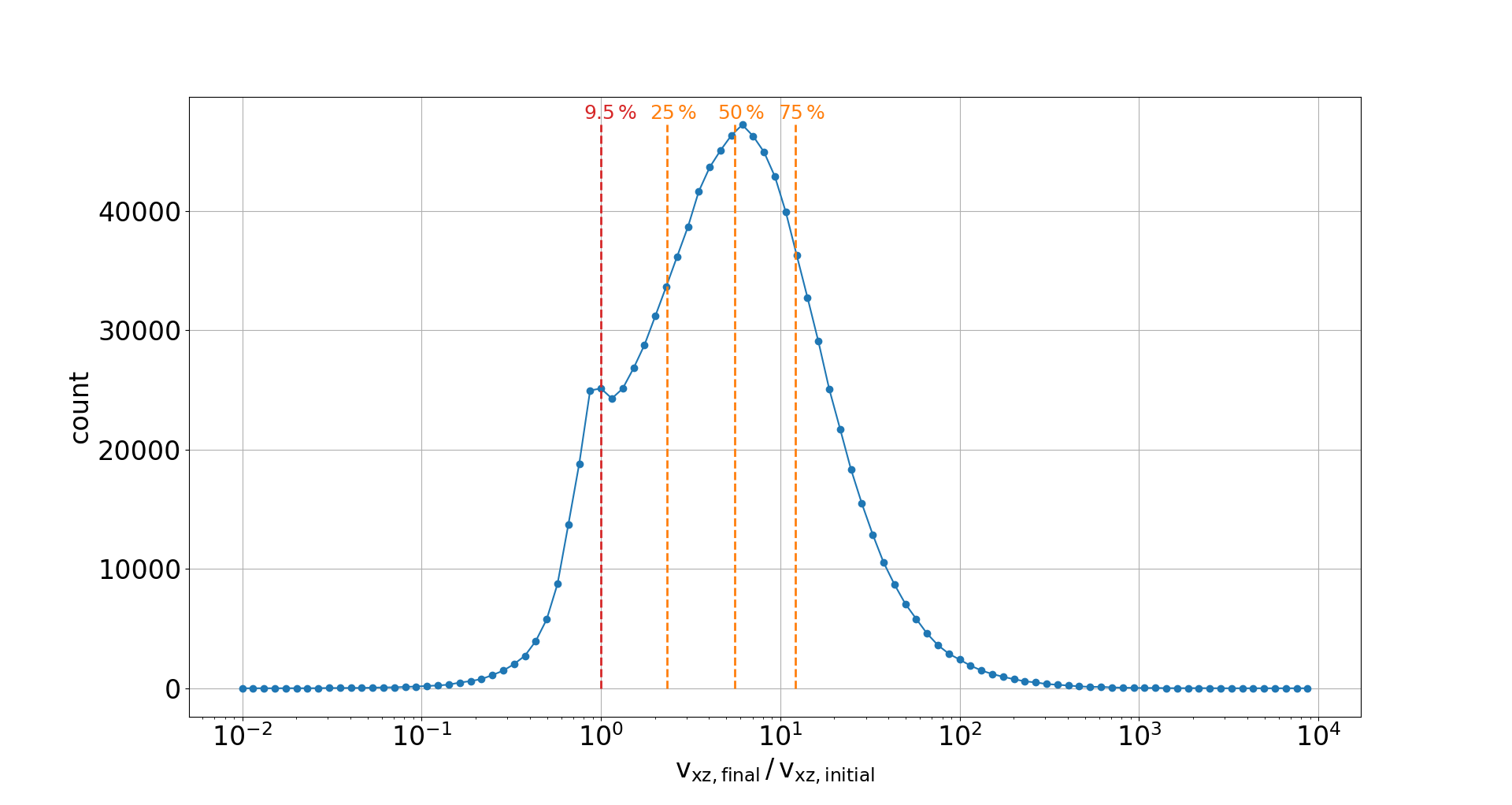
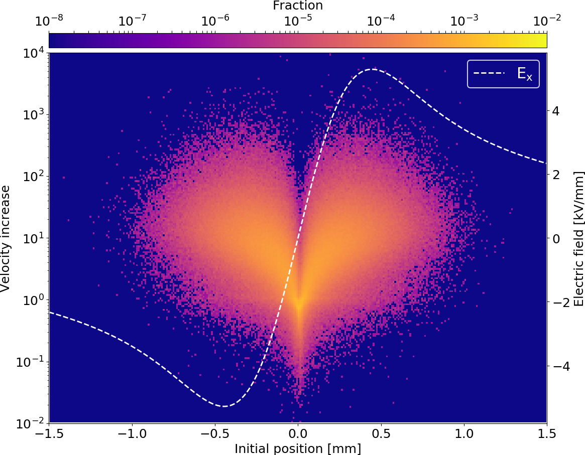
- This interaction effectively results in an increase of gyro-radii which consequently determines the profile distortion
- The increase itself depends on the starting position and thus on the bunch shape
🠖 prevents usage of simple description by other beam parameters (e.g. point-spread functions)
18/09/2018
3rd IPM Workshop, D. Vilsmeier
Profile distortion
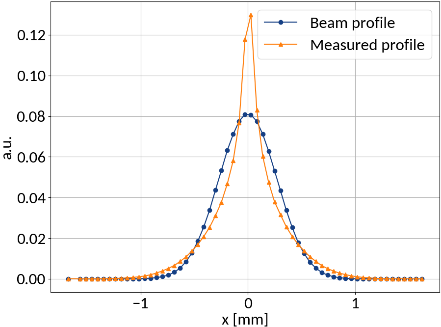
Ideally a one-dimensional projection the the transverse beam profile is measured, but...
\begin{aligned}
& E \; & 6.5 \, \textrm{TeV} \\
& N_q \; & 2.1\cdot 10^{11} \\
& \sigma_x \; & 0.27 \, \textrm{mm} \\
& \sigma_y \; & 0.36 \, \textrm{mm} \\
& 4\sigma_z \; & 0.9 \, \textrm{ns}
\end{aligned}
18/09/2018
3rd IPM Workshop, D. Vilsmeier
Magnetic field increase
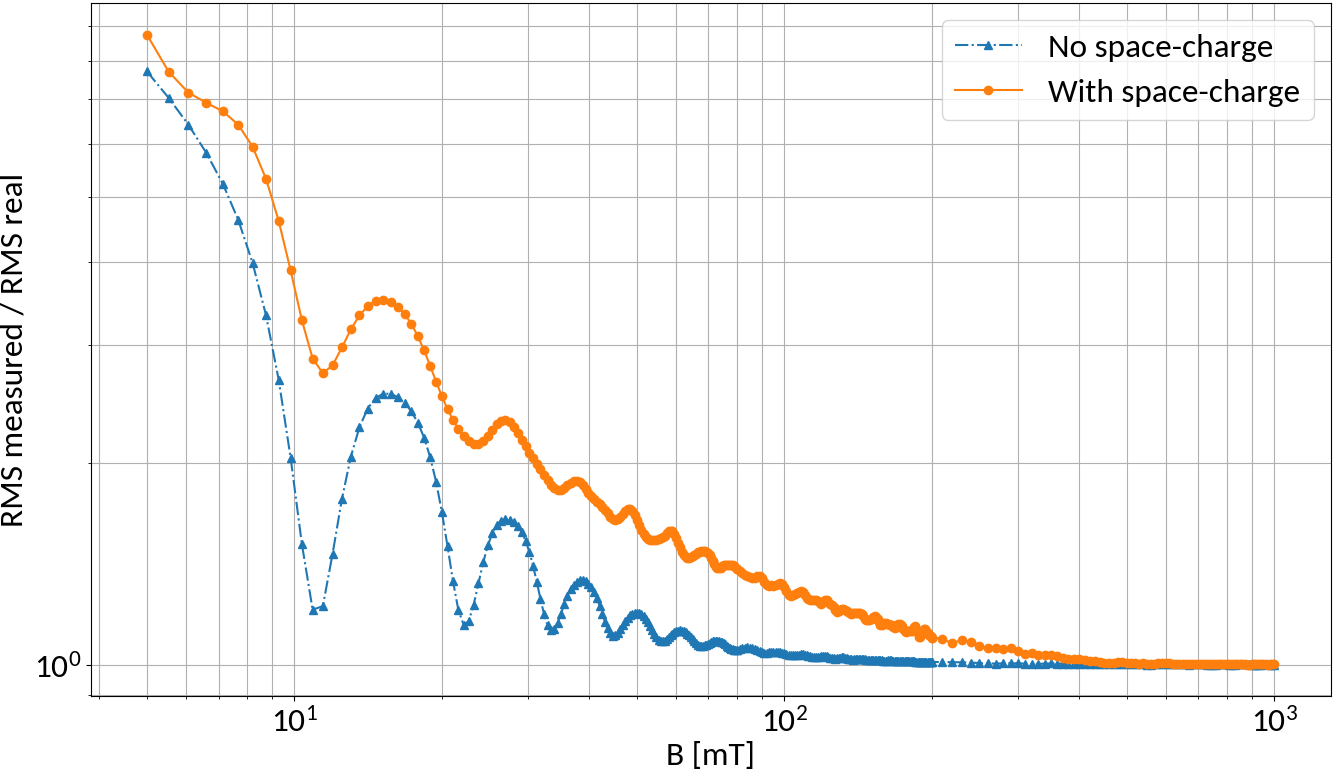
N-turn B-fields
Without space-charge electrons at the bunch center will perform exactly N turns for specific magnetic field strengths
Due to space-charge interaction only large field strengths are effective though
18/09/2018
3rd IPM Workshop, D. Vilsmeier
Using Machine Learning
| Parameter | Range | Step size |
|---|---|---|
| Bunch pop. [1e11] | 1.1 -- 2.1 ppb | 0.1 ppb |
| Bunch width (1σ) | 270 -- 370 μm | 5 μm |
| Bunch height (1σ) | 360 -- 600 μm | 20 μm |
| Bunch length (4σ) | 0.9 -- 1.2 ns | 0.05 ns |
Protons
6.5 TeV
4kV / 85mm
0.2 T
Training

Validation

Testing

Used to fit the model; split size ~ 60%.
Check generalization to unseen data; split size ~ 20%.
Evaluate final model performance; split size ~ 20%.
Consider 21,021 different cases
1
2
3
🠖 Evaluated on grid data and randomly sampled data
18/09/2018
3rd IPM Workshop, D. Vilsmeier
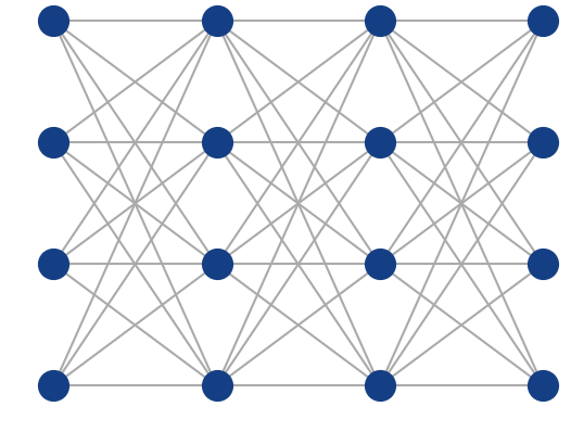
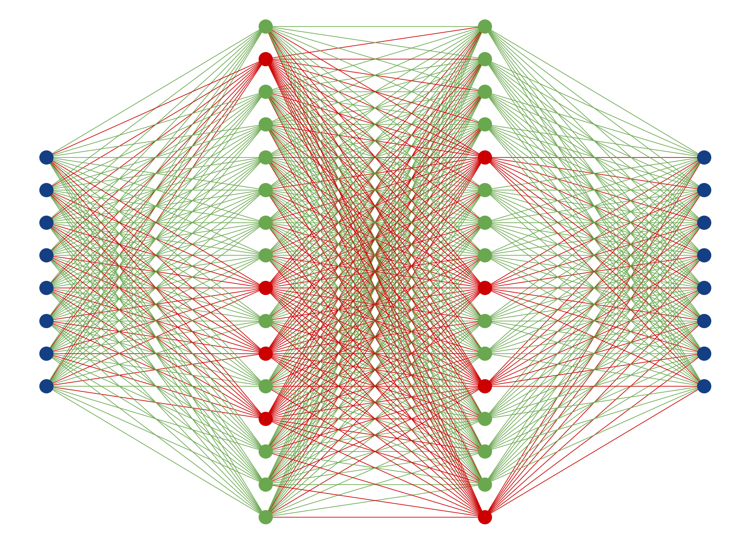
Artificial Neural Networks
Input layer
Weights
Bias
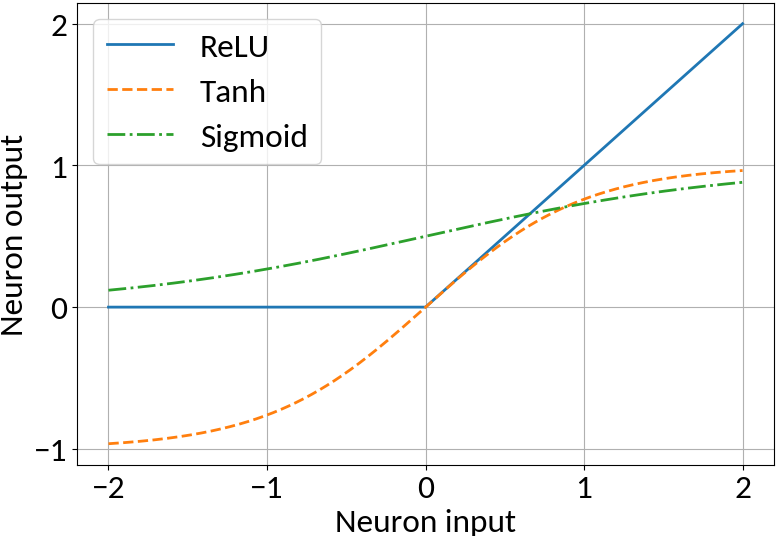
Apply non-linearity, e.g. ReLU, Tanh, Sigmoid
Perceptron
y(x) = \sigma\left( W\cdot x + b \right)
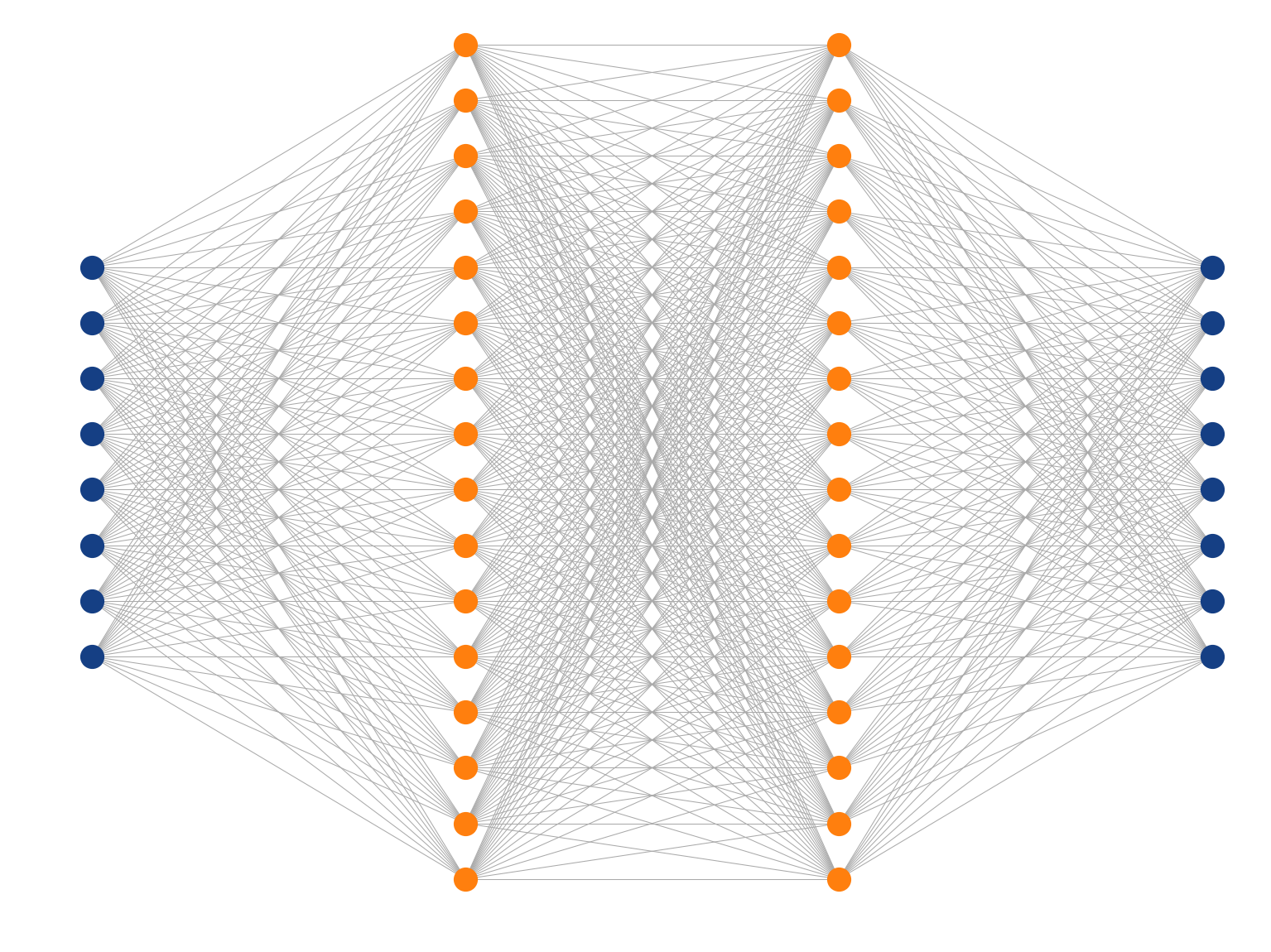
Multi-Layer Perceptron
Inspired by the human brain, many "neurons" linked together
Map non-linearities through non-linear activation functions
18/09/2018
3rd IPM Workshop, D. Vilsmeier
ANN Implementation
IDense = partial(Dense, kernel_initializer=VarianceScaling())

# Create feed-forward network.
model = Sequential()

# Since this is the first hidden layer we also need to specify
# the shape of the input data (49 predictors).
model.add(IDense(200, activation='relu', input_shape=(49,))
model.add(IDense(170, activation='relu'))
model.add(IDense(140, activation='relu'))
model.add(IDense(110, activation='relu'))

# The network's output (beam sigma). This uses linear activation.
model.add(IDense(1))
model.compile(
optimizer=Adam(lr=0.001),
loss='mean_squared_error'
)
model.fit(
x_train, y_train,
batch_size=8, epochs=100, shuffle=True,
validation_data=(x_val, y_val)
)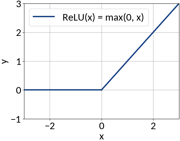
Fully-connected
feed-forward
network
with ReLU
activation
function
D. Kingma and J. Ba, "Adam: A Method for Stochastic Optimization", arXiv:1412.6980, 2014
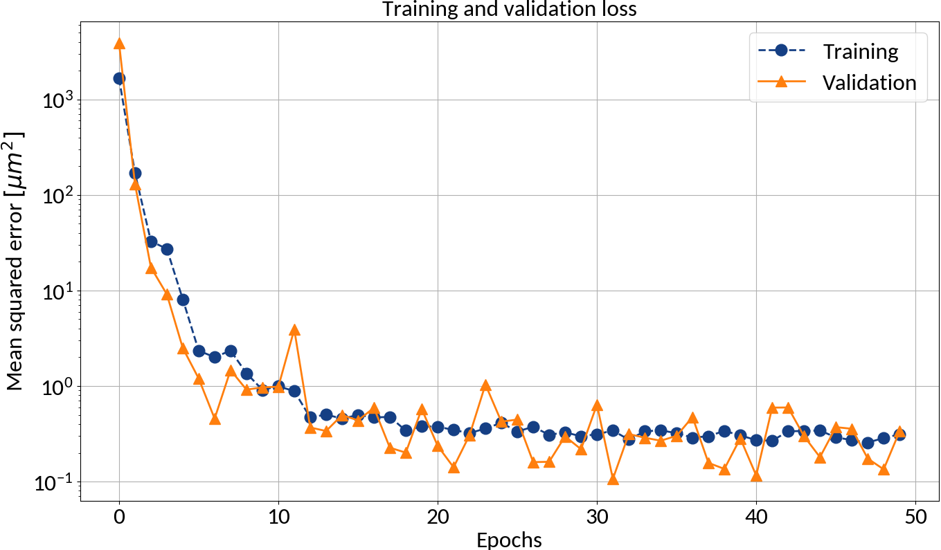
After each epoch compute loss on validation data in order to prevent "overfitting"
Batch learning
🠖 Iterate through training set multiple
times (= epochs)
🠖 Weight updates are performed in batches (of training samples)
keras
18/09/2018
3rd IPM Workshop, D. Vilsmeier
Why ANNs?
Universal approximation theorem
Every finite continuous "target" function can be approximated with arbitrarily small error by feed-forward network with single hidden layer
[corresponding Cybenko 1989; Hornik 1991]
y = \sum_j^n w_j^o \cdot \sigma\left( \sum_k^d w_{jk}^h x_k + b_j \right)
\(n\) hidden units
activation function
\(d\) - dimensional domain
parameters to be "optimized"
Proof of existence, i.e. no universal optimization algorithm exists 🠖 "No free lunch theorem"
Works on compact subsets of \(\mathbb{R}^d\)
18/09/2018
3rd IPM Workshop, D. Vilsmeier
Profile RMS Inference - Results
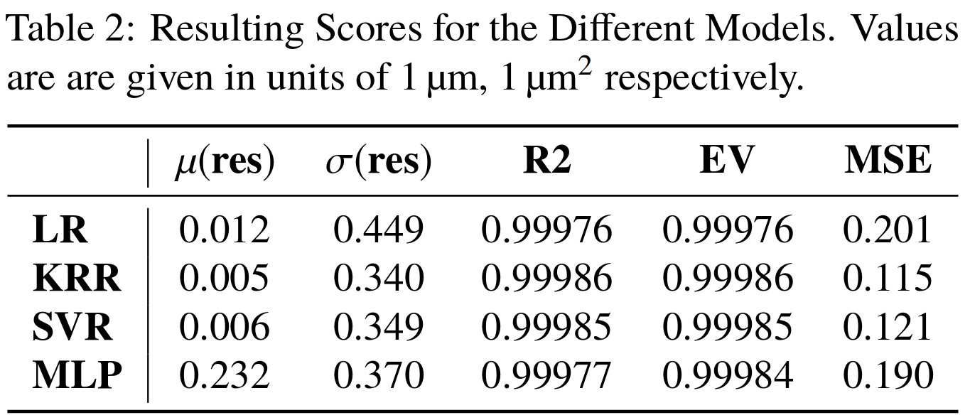
Tested also other machine learning algorithms:
• Linear regression (LR)
• Kernel ridge regression (KRR)
• Support vector machine (SVR)
Multi-layer perceptron (= ANN)
Very good results on simulation data 🠖 below 1% accuracy
Results are without consideration of noise on profile data
18/09/2018
3rd IPM Workshop, D. Vilsmeier
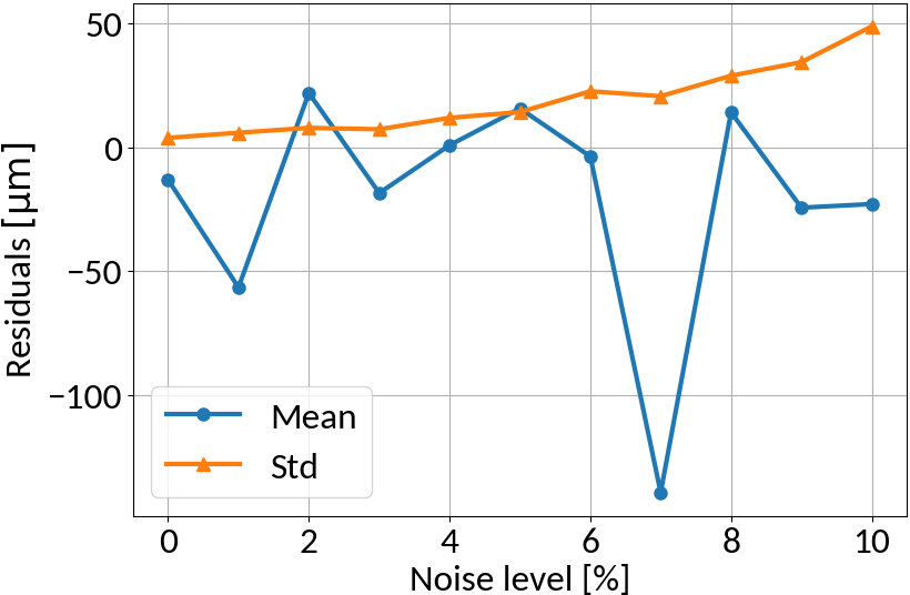
RMS Inference with Noise
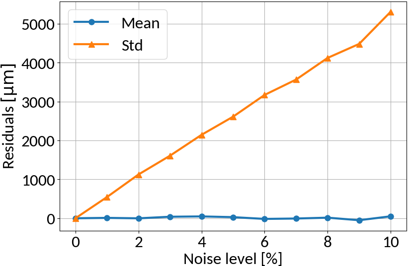
Linear regression model
no noise on training data
similar noise on training data
Linear regression amplifies noise in predictions if not explicitly trained
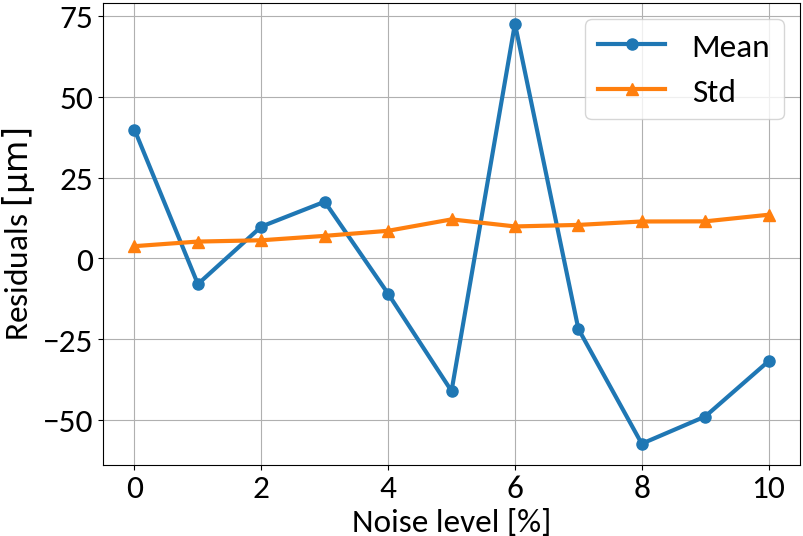
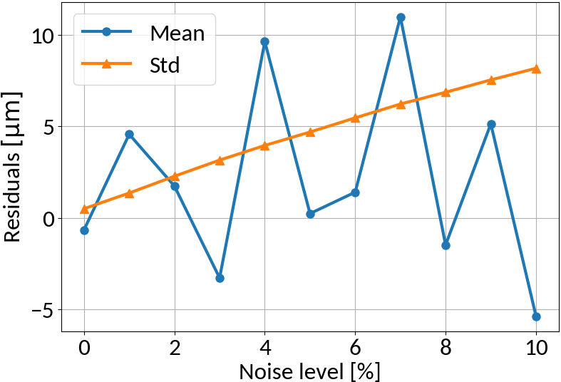
Multi-layer perceptron
MLP amplifies noise; bounded activation functions could help; as well as duplicating data before "noising"
18/09/2018
3rd IPM Workshop, D. Vilsmeier
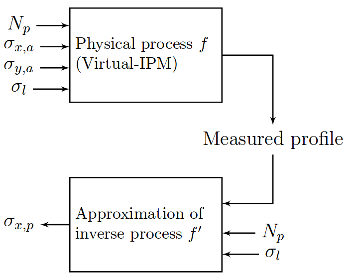
Full Profile Reconstruction
So far:
Machine Learning Model
\sigma_z
N
\sigma_x
Instead:
Machine Learning Model
\sigma_z
N
Compute beam RMS
Compute beam profile
18/09/2018
3rd IPM Workshop, D. Vilsmeier
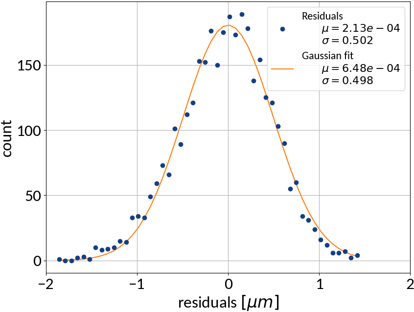
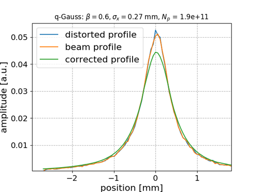
Gaussian bunch shape
MLP Architecture
- 2 hidden layers, 88 nodes
-
tanh activation function
Performance measure
- Mean squared error (MSE)
\textrm{MSE} = \frac{1}{N}\sum_{i=1}^{N}\left( y_{p,i} - y_{i} \right)^2
prediction
target
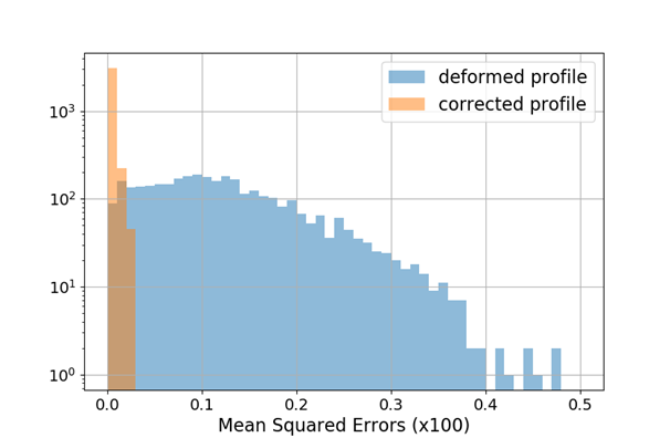
\begin{aligned}
\textrm{mean} &= 0.1231 \\
\textrm{std} &= 0.0808
\end{aligned}
\begin{aligned}
\textrm{mean} &= 0.0024 \\
\textrm{std} &= 0.0045
\end{aligned}
18/09/2018
3rd IPM Workshop, D. Vilsmeier
Generalized Gaussian bunch shape
\frac{\beta}{2\alpha\Gamma(1/\beta)}e^{-\left(\lvert x-\mu\rvert/\alpha\right)^{\beta}}
Gen-Gauss used for testing while training (fitting) was performed with Gaussian bunch shape
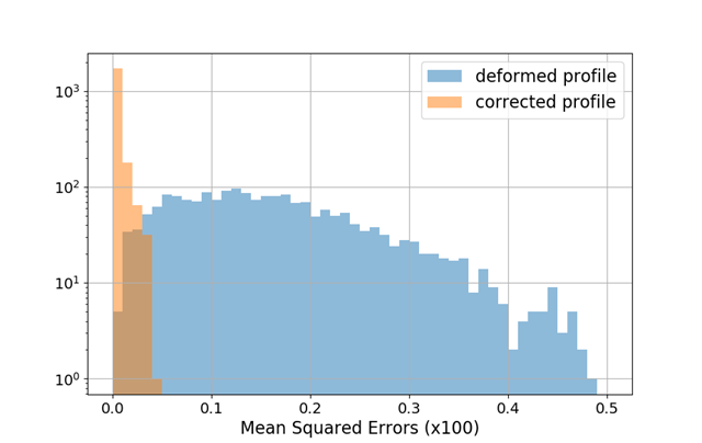
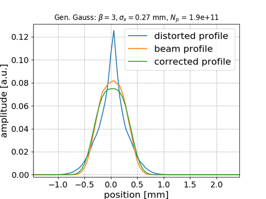
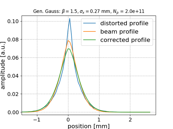
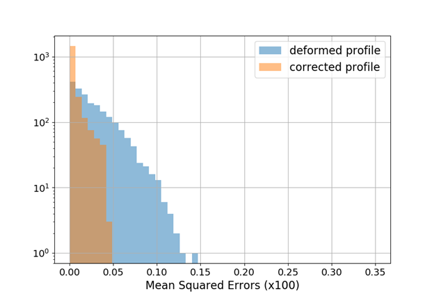
\beta = 3
\beta = 1.5
Smaller distortion in this case
\begin{aligned}
\textrm{mean} &= 0.0278 \\
\textrm{std} &= 0.0237
\end{aligned}
\begin{aligned}
\textrm{mean} &= 0.0068 \\
\textrm{std} &= 0.0087
\end{aligned}
\begin{aligned}
\textrm{mean} &= 0.1638 \\
\textrm{std} &= 0.0974
\end{aligned}
\begin{aligned}
\textrm{mean} &= 0.0051 \\
\textrm{std} &= 0.0064
\end{aligned}
ANN model generalizes to different beam shapes
18/09/2018
3rd IPM Workshop, D. Vilsmeier
Q-Gaussian bunch shape
\frac{\sqrt{\beta}}{C_q}\left[1 - (1 - q)\beta x^2\right]^{\frac{1}{1-q}}
Q-Gauss used for testing while training (fitting) was performed with Gaussian bunch shape
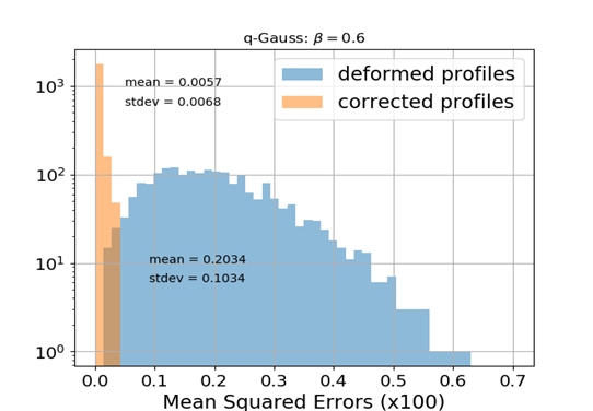
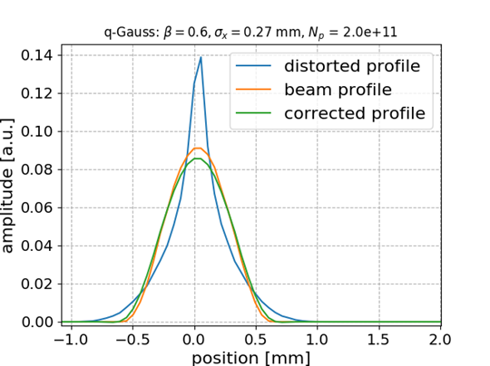
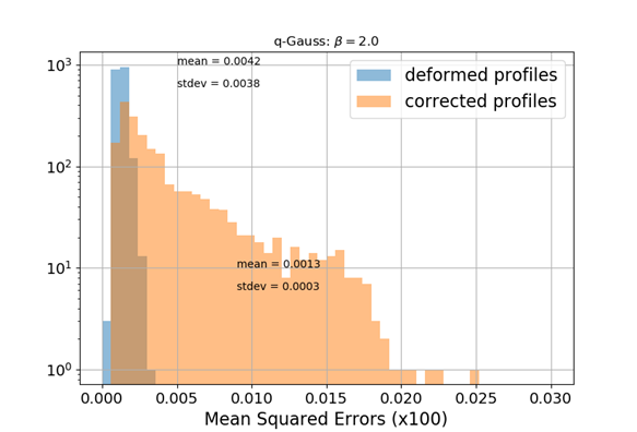
q = 0.6
q = 2.0
\begin{aligned}
\textrm{mean} &= 0.0013 \\
\textrm{std} &= 0.0003
\end{aligned}
\begin{aligned}
\textrm{mean} &= 0.0042 \\
\textrm{std} &= 0.0038
\end{aligned}
\begin{aligned}
\textrm{mean} &= 0.2034 \\
\textrm{std} &= 0.1034
\end{aligned}
\begin{aligned}
\textrm{mean} &= 0.0057 \\
\textrm{std} &= 0.0068
\end{aligned}
No distortion for this case
🠖 nothing to correct for; MLP preserves the state
ANN model generalizes to different beam shapes
18/09/2018
3rd IPM Workshop, D. Vilsmeier
Model prediction uncertainty
- Could train multiple models with different initialization and different data presentation 🠖 ensemble of predictions
- Emulate multi-model ensemble by using "Dropout" layers (also for predictions)
inactive
active
MLP shows very small standard deviation in predictions 🠖 the fitting converged well, small model uncertainty
\pm 1\sigma
18/09/2018
3rd IPM Workshop, D. Vilsmeier
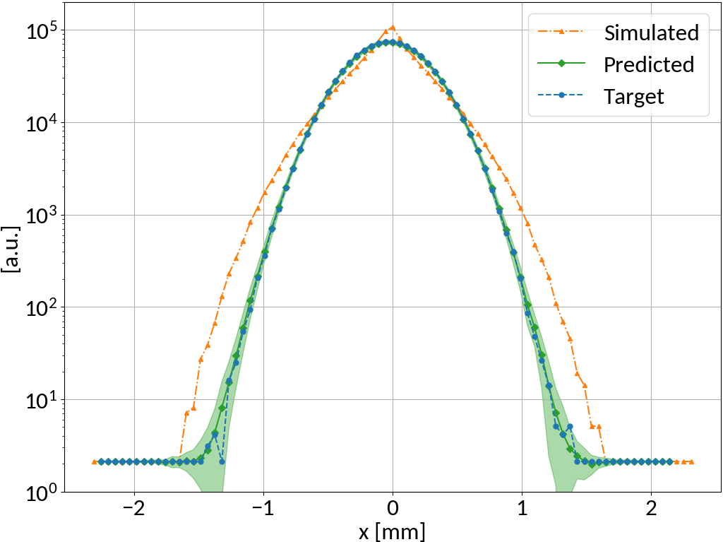
Sub-resolution measurements
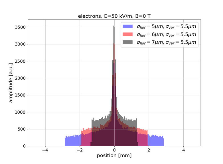
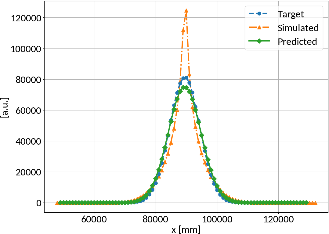
- Understanding or (machine) "learning" beam profile deformation (and how to revert it), this information could be used to measure beams that are smaller than the resolution of the detector (by provoking a deformation / blow-up, then reverting it)
- Example: SwissXFEL, 5.8 GeV electrons, 230 pC bunch charge, 21 fs bunch length, 5-7 μm transverse size
- Bunch size is 1/10-th of detector resolution however the deformed profile is well above and strongly depends on the bunch size
- Alternative to R. Tarkeshian et al. Phys. Rev. X 8, 021039 (reconstruction based on ion energies)
preliminary
18/09/2018
3rd IPM Workshop, D. Vilsmeier
Summary
- Successful beam RMS reconstruction with various machine learning models
- Reconstruction of complete profiles with multi-layer perceptron model
- The mapping generalizes to different beam shapes
- Model seems to "learn" the distortion mechanisms rather than specific beam shapes
- Model uncertainty estimates show small variations
- These methods could potentially be used to measure sub-resolution beam profiles
Icons by icons8.
Resolving Profile Distortion for Electron-based IPMs using Machine Learning
By Dominik Vilsmeier
Resolving Profile Distortion for Electron-based IPMs using Machine Learning
International workshop on non-invasive beam profile monitors for hadron machines and its related techniques: 3rd IPM workshop, Japan Proton Accelerator Research Complex (Tokai, Japan), September 18th 2018


