Deep Probabilistic Learning
in JAX/Flax and TensorFlow Probability
Francois Lanusse @EiffL
+ p(x) =


Advanced Euclid School, June 2022
Learning Objectives for this Session
- How to write and train a Neural Network in JAX/Flax
- Understanding the probabilistic meaning of common loss functions
- How to merge Neural Networks with Probabilities
Our case study
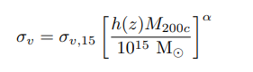
Dynamical Mass Measurement for Galaxy Clusters
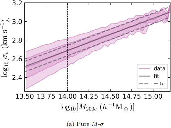
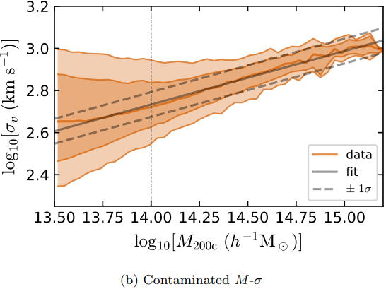
Figures and data from Ho et al. 2019
Our Goal: Train a Neural Network to Estimate Cluster Masses
What we will feed the model:
- Richness
- Velocity Dispersion
- Information about member galaxies:
- radial distribution
- stellar mass distribution
- LOS velocity distribution
What kind of uncertainties should I most worry about?
- Epistemic
- Aleatoric
Training data from MultiDark Planck 2 N-body simulation (Klypin et al. 2016) with 261287 clusters.
Different Sources of Uncertainties
From this excellent tutorial:
- Linear regression
- Aleatoric Uncertainties
- Epistemic Uncertainties
- Epistemic+ Aleatoric Uncertainties
\hat{y} = a x
\hat{y} \sim \mathcal{N}(a x, \sigma^2)
\hat{y} = w x \quad w \sim p(w | \{x_i, y_i\})
\hat{y} \sim \mathcal{N}(w x, \sigma^2) \\ w, \sigma \sim p(w, \sigma | \{x_i, y_i\})
Why JAX?
and what is it?


JAX: NumPy + Autograd + XLA
- JAX uses the NumPy API
=> You can copy/paste existing code, works pretty much out of the box
- JAX is a successor of autograd
=> You can transform any function to get forward or backward automatic derivatives (grad, jacobians, hessians, etc)
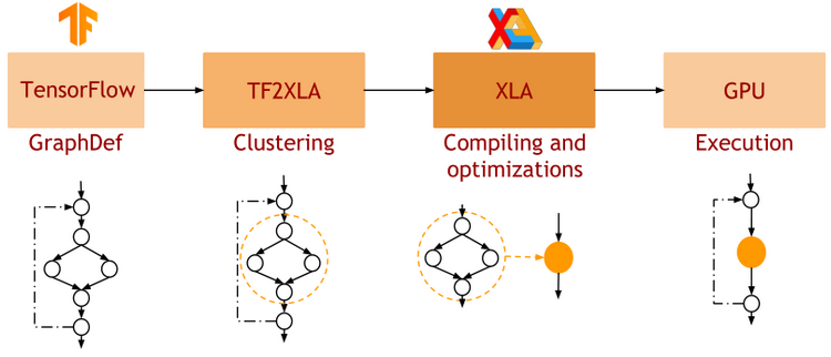
- JAX uses XLA as a backend
=> Same framework as used by TensorFlow (supports CPU, GPU, TPU execution)
import jax.numpy as np

m = np.eye(10) # Some matrix

def my_func(x):
  return m.dot(x).sum()

x = np.linspace(0,1,10)
y = my_func(x)
from jax import grad
df_dx = grad(my_func)
y = df_dx(x)
-
Pure functions
=> JAX is designed for functional programming: your code should be built around pure functions (no side effects)- Enables caching functions as XLA expressions
- Enables JAX's extremely powerful concept of composable function transformations
-
Just in Time (jit) Compilation
=> jax.jit() transformation will compile an entire function as XLA, which then runs in one go on GPU.
-
Arbitrary order forward and backward autodiff
=> jax.grad() transformation will apply the d/dx operator to a function f
-
Auto-vectorization
=> jax.vmap() transformation will add a batch dimension to the input/output of any function
def pure_fun(x):
  return 2 * x**2 + 3 * x + 2


def impure_fun_side_effect(x):
  print('I am a side effect')
  return 2 * x**2 + 3 * x + 2


C = 10. # A global variable
def impure_fun_uses_globals(x):
  return 2 * x**2 + 3 * x + C
# Decorator for jitting
@jax.jit
def my_fun(W, x):
return W.dot(x)
# or as an explicit transformation
my_fun_jitted = jax.jit(my_fun)def f(x):
return 2 * x**2 + 3 *x + 2
df_dx = jax.grad(f)
jac = jax.jacobian(f)
hess = jax.hessian(f)
# As decorator
@jax.vmap
def f(x):
  return 2 * x**2 + 3 *x + 2

# Can be composed
df_dx = jax.jit(jax.vmap(jax.grad(f)))
Writing a Neural Network in JAX/Flax
import flax.linen as nn
import optax

class MLP(nn.Module):
  @nn.compact
  def __call__(self, x):
    x = nn.relu(nn.Dense(128)(x))
    x = nn.relu(nn.Dense(128)(x))
    x = nn.Dense(1)(x)
    return x
# Instantiate the Neural Network
model = MLP()
# Initialize the parameters
params = model.init(jax.random.PRNGKey(0), x)
prediction = model.apply(params, x)
# Instantiate Optimizer
tx = optax.adam(learning_rate=0.001)
opt_state = tx.init(params)
# Define loss function
def loss_fn(params, x, y):
  mse = model.apply(params, x) -y)**2
  return jnp.mean(mse)
# Compute gradients
grads = jax.grad(loss_fn)(params, x, y)
# Update parameters
updates, opt_state = tx.update(grads, opt_state)
params = optax.apply_updates(params, updates)- Model Definition: Subclass the flax.linen.Module base class. Only need to define the __call__() method.
-
Using the Model: the model instance provides 2 important methods:
- init(seed, x): Returns initial parameters of the NN
- apply(params, x): Pure function to apply the NN
- Training the Model: Use jax.grad to compute gradients and Optax optimizers to update parameters
Now You Try it!
We will be using this notebook
Your goal: Building a regression model with a Mean Squared Error loss in JAX/Flax
def loss_fn(params, x, y):
  mse = model.apply(params, x) -y)**2
  return jnp.mean(mse)
Raise your hand when you reach the cluster mass prediction plot
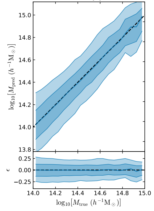
First attempt with an MSE loss
class MLP(nn.Module):
  @nn.compact
  def __call__(self, x):
    x = nn.relu(nn.Dense(128)(x))
    x = nn.relu(nn.Dense(128)(x))
    x = nn.tanh(nn.Dense(64)(x))
    x = nn.Dense(1)(x)
    return x

def loss_fn(params, x, y):
  prediction = model.apply(params, x)
  return jnp.mean( (prediction - y)**2 )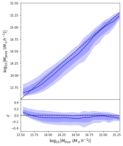
- Simple Dense network using 14 features derived from galaxy positions and velocity information
- We see that the predictions are biased compared to the true value of the mass... Not good.
What is going on???

Let's try to understand the neural network output by looking at the loss function
$$ \mathcal{L} = \sum_{(x_i, y_i) \in \mathcal{D}} \parallel y_i - f_\theta(x_i)\parallel^2 \quad \simeq \quad \int \parallel y - f_\theta(x) \parallel^2 \ p(x,y) \ dx dy $$ $$\Longrightarrow \int \left[ \int \parallel y - f_\theta(x) \parallel^2 \ p(y|x) \ dy \right] p(x) dx$$
This is minimized when $$f_{\theta^\star}(x) = \int y \ p(y|x) \ dy $$
i.e. when the network is predicting the mean of p(y|x).
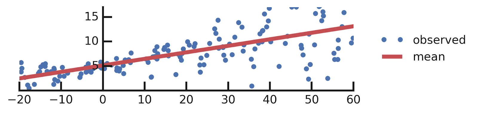
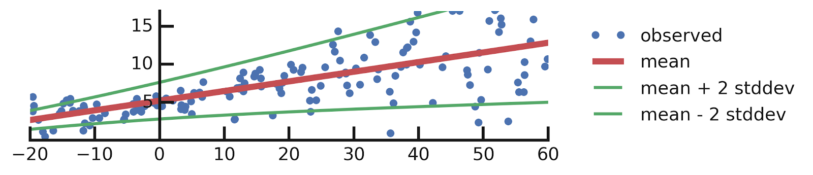
A Probabilistic Understanding of MSE training
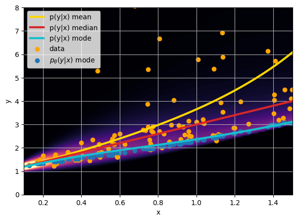
Let us consider a toy regression example
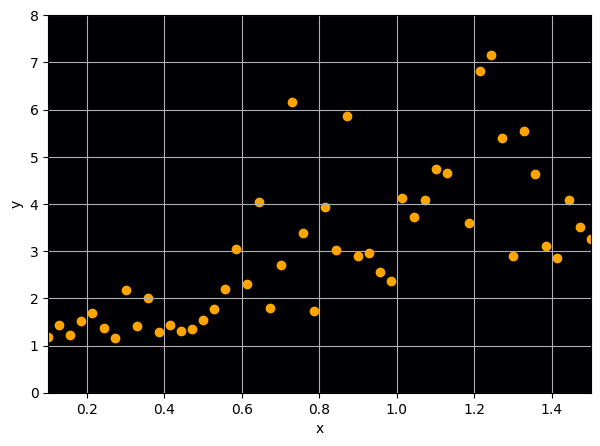
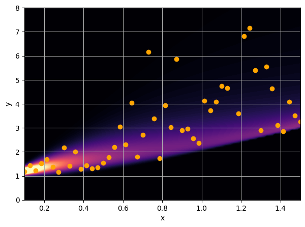
There are intrinsic uncertainties in this problem, at each x there is a full
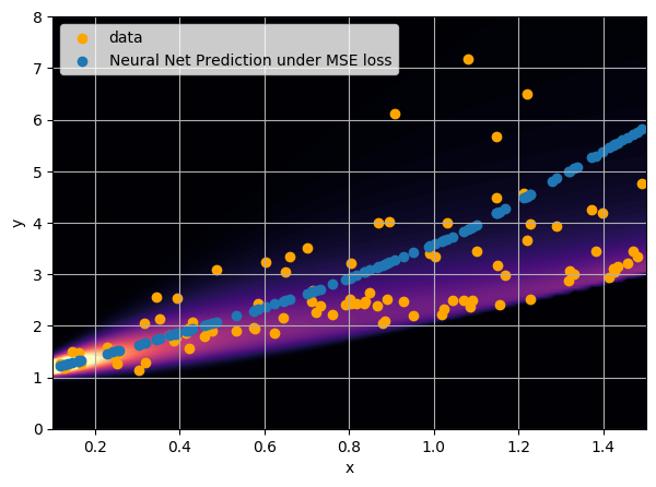
- Option 1) Train a neural network to learn a function under an MSE loss:
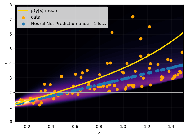
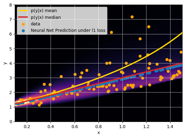
- Option 2) Train a neural network to learn a function under an l1 loss:
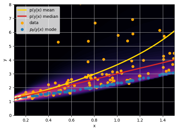
- Option 3) Train a neural network to learn a distribution using a Maximum Likelihood loss
\hat{y} = f_\varphi(x)
\mathcal{L} = \parallel y - f_\varphi(x) \parallel_2^2
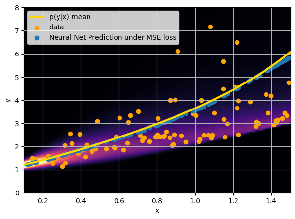
p(y | x)
I have a set of data points {x, y} where I observe x and want to predict y.
\hat{y} = f_\varphi(x)
\mathcal{L} = | y - f_\varphi(x) |
p_\varphi(y | x)
\mathcal{L} = - \log p_\varphi(y | x )
q_\varphi(\theta= \mathrm{cat} | x) = 0.9
x
credit: Venkatesh Tata
Let's start with binary classification
\theta
=> This means expressing the posterior as a Bernoulli distribution with parameter predicted by a neural network
How do we adjust this parametric distribution to match the true posterior ?
Step 1: We neeed some data
\mathcal{D} = \{ (x_i, \theta_i) \}_{i \in [0, N]}
cat or dog image
label 1 for cat, 0 for dog
(x, \theta) \sim p(x, \theta) = p(\theta) p(x | \theta)
Probability of including cats and dogs in my dataset
Implicit prior
Image search results for cats and dogs
Implicit likelihood
A distance between distributions: the Kullback-Leibler Divergence
D_{KL} (p || q) = \mathbb{E}_{x \sim p(x)} \left[ \log \frac{p(x)}{q(x)} \right]
Step 2: We need a tool to compare distributions
D_{KL} \left( p(x, \theta) || q_\varphi(\theta| x) p(x) \right) = - \mathbb{E}_{p(x,\theta)} \left[ \log \frac{ q_\varphi(\theta | x) p(x) }{ p(x) p(\theta | x) } \right]
= - \mathbb{E}_{p(x, \theta)} \left[ \log q_\varphi(\theta | x) \right] + cst
Minimizing this KL divergence is equivalent to minimizing the negative log likelihood of the model
D_{KL} \left( p(x, \theta) || q_\varphi(\theta | x) p(x) \right) = 0
\\
<=>
\\
q_\varphi(\theta | x) = p(\theta | x)
In our case of binary classification:
\mathbb{E}_{p(x,\theta)}[ - \log q_\varphi(\theta | x)] =\\ \sum_{i=1}^{N} p(1|x_i) \log q_\varphi(1 | x_i) + (1-p(1|x_i)) \log_\varphi(1 | x_i)
We recover the binary cross entropy loss function !
The Probabilistic Deep Learning Recipe
- Express the output of the model as a distribution
- Optimize for the negative log likelihood
- Maybe adjust by a ratio of proposal to prior if the training set is not distributed according to the prior
- Profit!
q_\varphi(\theta | x)
\mathcal{L} = - \log q_\varphi(\theta | x)
q_\varphi(\theta | x) \propto \frac{\tilde{p}(\theta)}{p(\theta)} p(\theta | x)
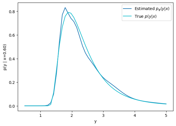
How do we model more complex distributions?
We need a parametric conditional distribution to
compute
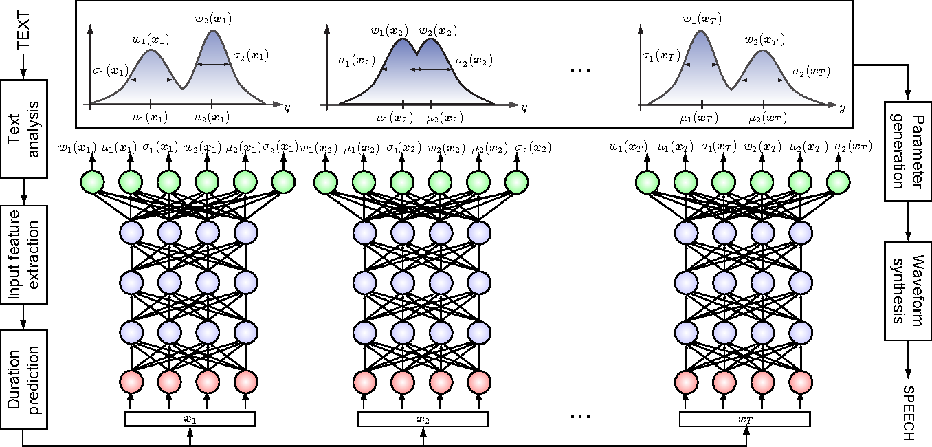
- Mixture Density Networks
Bishop 1994
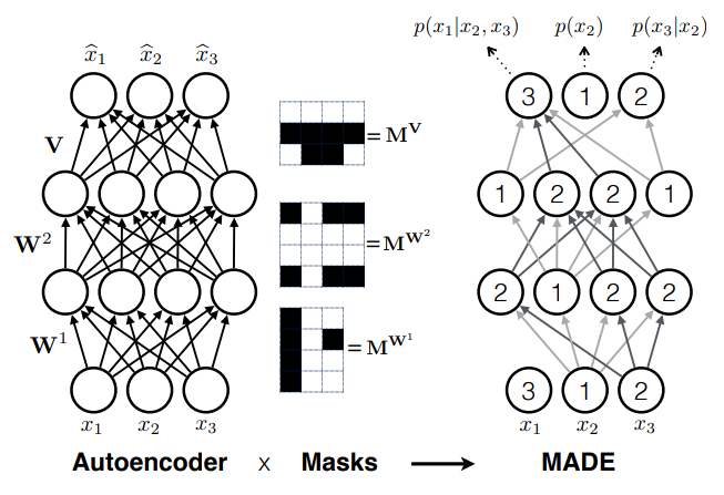
- Autoregressive models
e.g. MADE (Germain et al. 2015)
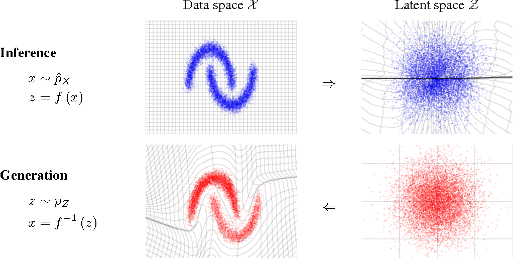
- Normalizing Flows
e.g. MAF (Papamakarios et al. 2017)
\log p_\varphi(y | x)
p_\varphi(y | x) = \sum_{i=1}^K \pi_i \mathcal{N}( \mu_\varphi(x), \Sigma_\varphi(x))
p_\varphi(y | x) = \Pi_{d=1}^D p_\varphi(y_d | y_1, \ldots, y_{d-1}, x)
p_\varphi(y | x) = p(z = f_\varphi(y, x)) \left| \det \frac{\partial f_\varphi}{\partial z} \right|
Let's build a Conditional Density Estimator with TFP
class MDN(nn.Module):
  num_components: int

  @nn.compact
  def __call__(self, x):
    x = nn.relu(nn.Dense(128)(x))
    x = nn.relu(nn.Dense(128)(x))
    x = nn.tanh(nn.Dense(64)(x))

    # Instead of regressing directly the value of the mass, the network
    # will now try to estimate the parameters of a mass distribution.
    categorical_logits = nn.Dense(self.num_components)(x)
    loc = nn.Dense(self.num_components)(x)
    scale = 1e-3 + nn.softplus(nn.Dense(self.num_components)(x))

    dist =tfd.MixtureSameFamily(
        mixture_distribution=tfd.Categorical(logits=categorical_logits),
        components_distribution=tfd.Normal(loc=loc, scale=scale))

    # To make it understand the batch dimension
    dist =  tfd.Independent(dist)

    # Returns a distribution !
    return dist
Now you try it!
Your goal: Implement a Mixture Density Network in JAX/Flax/TFP, and use it to get unbiased mass estimates.
When everyone is done, we will discuss the results.
def loss_fn(params, x, y):
  q = model.apply(params, x)
  return jnp.mean( - q.log_prob(y[:,0]) )
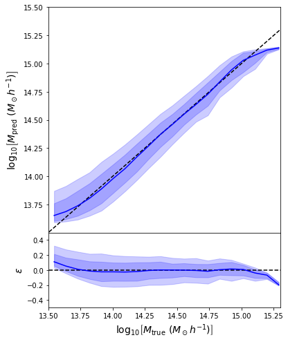
Second attempt: Probabilistic Modeling
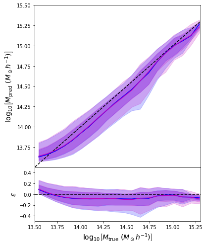
- Same Dense network but now using a Mixture Density output.
- Using the mean of the predicted distribution as our mass estimate: We see the exact same behaviour
What am I doing wrong???
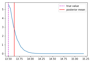
Accounting for Implicit Prior
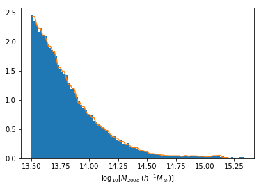
Distribution of masses in our training data

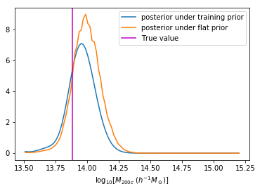
q(M_{200c} | x ) \propto \frac{\tilde{p}(M_{200c})}{p(M_{200c})} p(M_{200c} | x)
We can reweight the predictions for a desired prior
Last detail, use the mode instead of the mean posterior
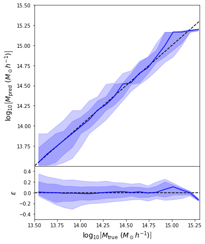
Takeaway Message
- Using a model that outputs distributions instead of scalars is always better!
- It's 2 lines of TensorFlow Probability
- Careful about interpreting these distributions as a Bayesian posterior, the training set acts as an Interim Prior, not necessarily matching your Bayesian prior.
=> Connection with proper Simulation Based Inference by Neural Density Estimation
A brief Mention of How to Model Epistemic Uncertainties
A Quick reminder
From this excellent tutorial:
- Linear regression
- Aleatoric Uncertainties
- Epistemic Uncertainties
- Epistemic+ Aleatoric Uncertainties
\hat{y} = a x
\hat{y} \sim \mathcal{N}(a x, \sigma^2)
\hat{y} = w x \quad w \sim p(w | \{x_i, y_i\})
\hat{y} \sim \mathcal{N}(w x, \sigma^2) \\ w, \sigma \sim p(w, \sigma | \{x_i, y_i\})
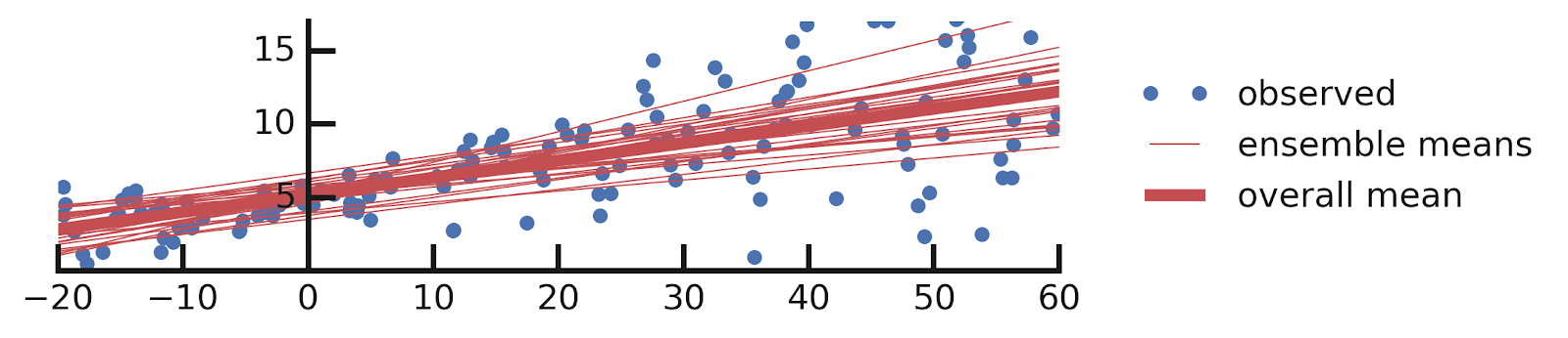
The idea behind Bayesian Neural Networks
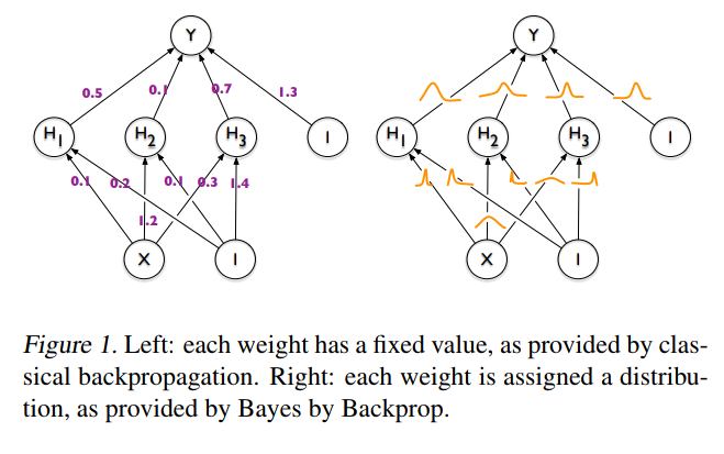
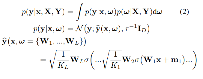
Given a training set D = {X,Y}, the predictions from a Neural Network can be expressed as:
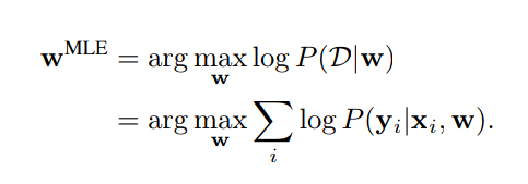
Weight Estimation by Maximum Likelihood
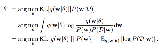
Weight Estimation by Variational Inference
A first approach to BNNs:
Bayes by Backprop (Blundel et al. 2015)
-
Step 1: Assume a variational distribution for the weights of the Neural Network
-
Step 2: Assume a prior distribution for these weights
- Step 3: Learn the parameters of the variational distribution by minimizing the ELBO
q_\theta(w) = \mathcal{N}( \mu_\theta, \Sigma_\theta )
p(w) = \mathcal{N}(0, I)
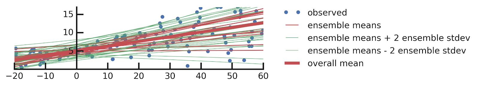
What happens in practice
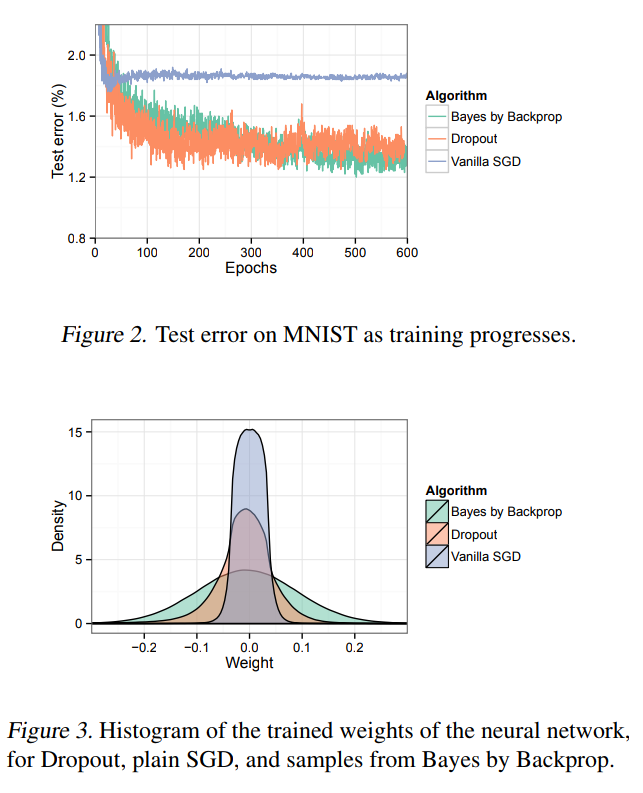
TensorFlow Probability implementation
A different approach:
Dropout as a Bayesian Approximation (Gal & Ghahramani, 2015)
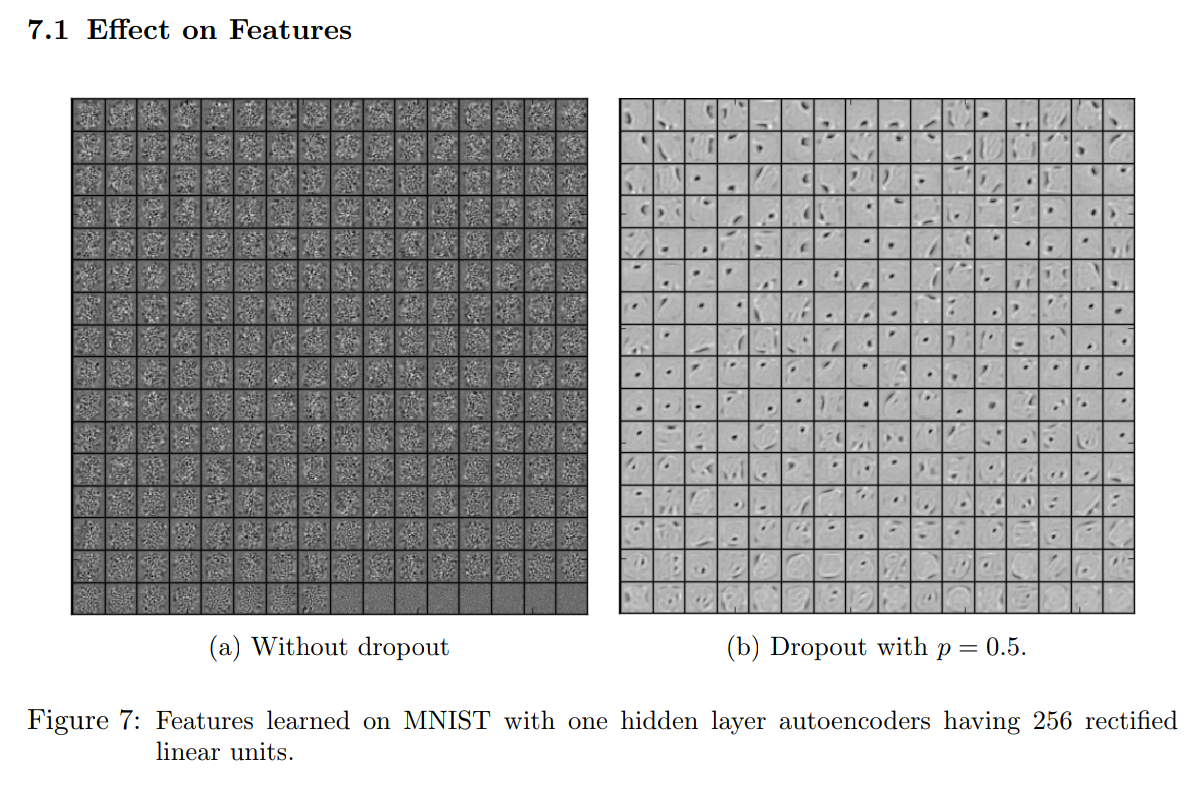
Quick reminder on dropout
Hinton 2012, Srivastava 2014

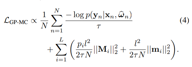
Variational Distribution of Weights under Dropout
-
Step 1: Assume a Variational Distribution for the weights
-
Step 2: Assume a Gaussian prior for the weights, with "length scale" l
- Step 3: Fit the parameters of the variational distribution by optimizing the ELBO

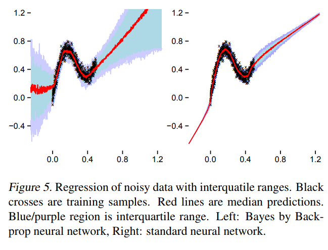
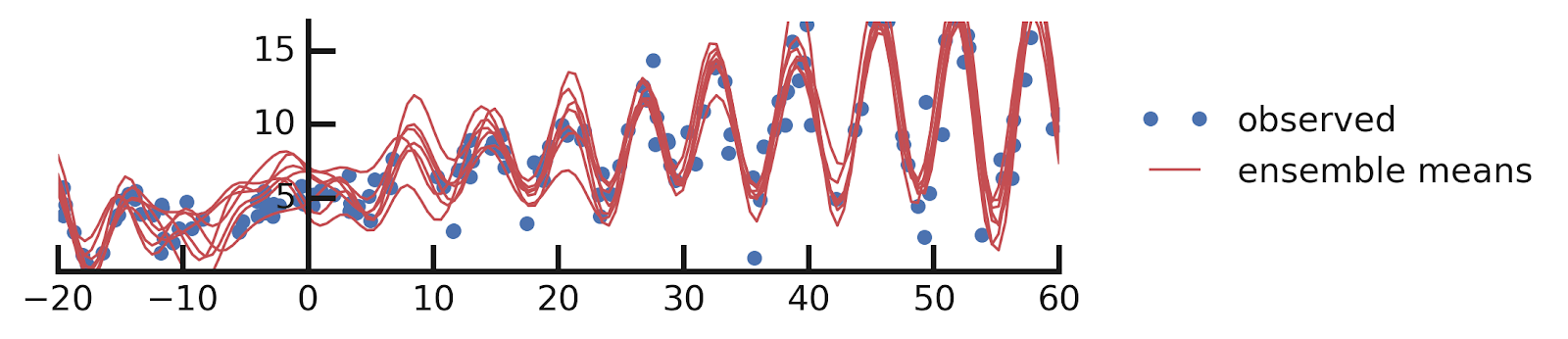
Example
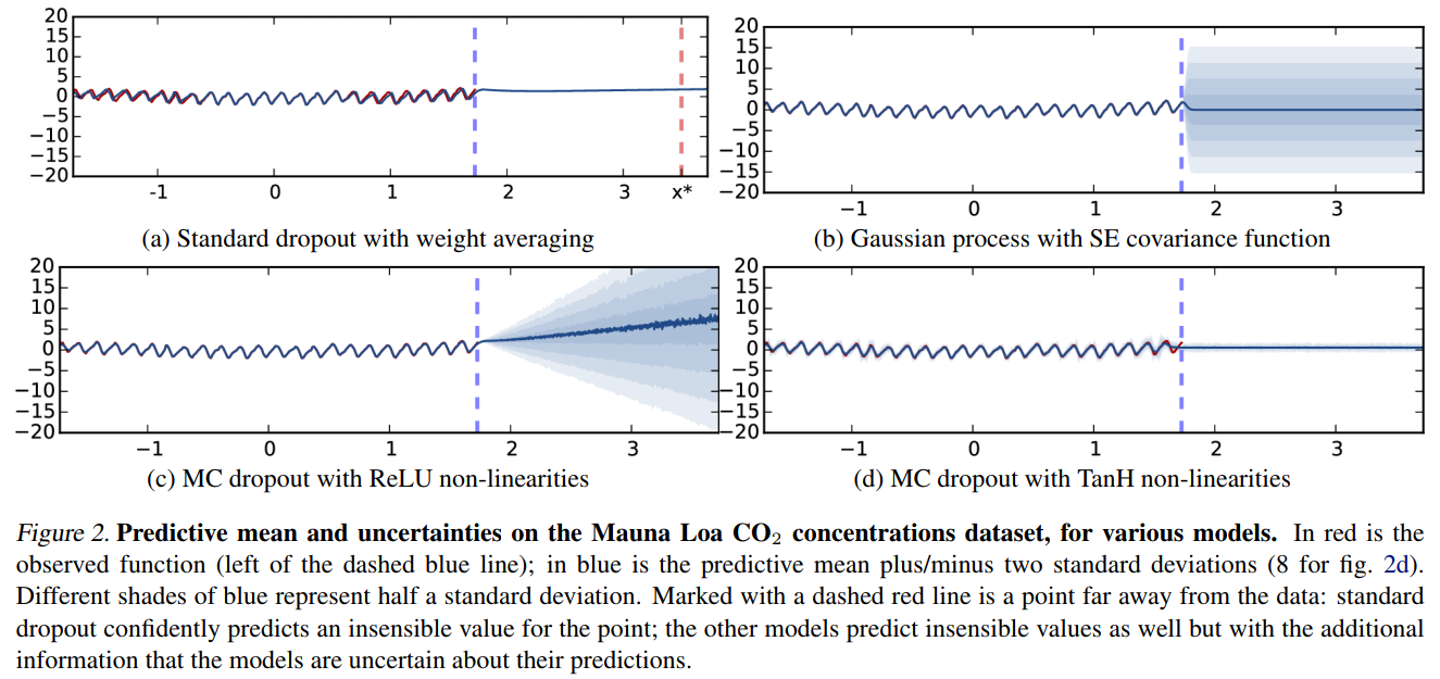
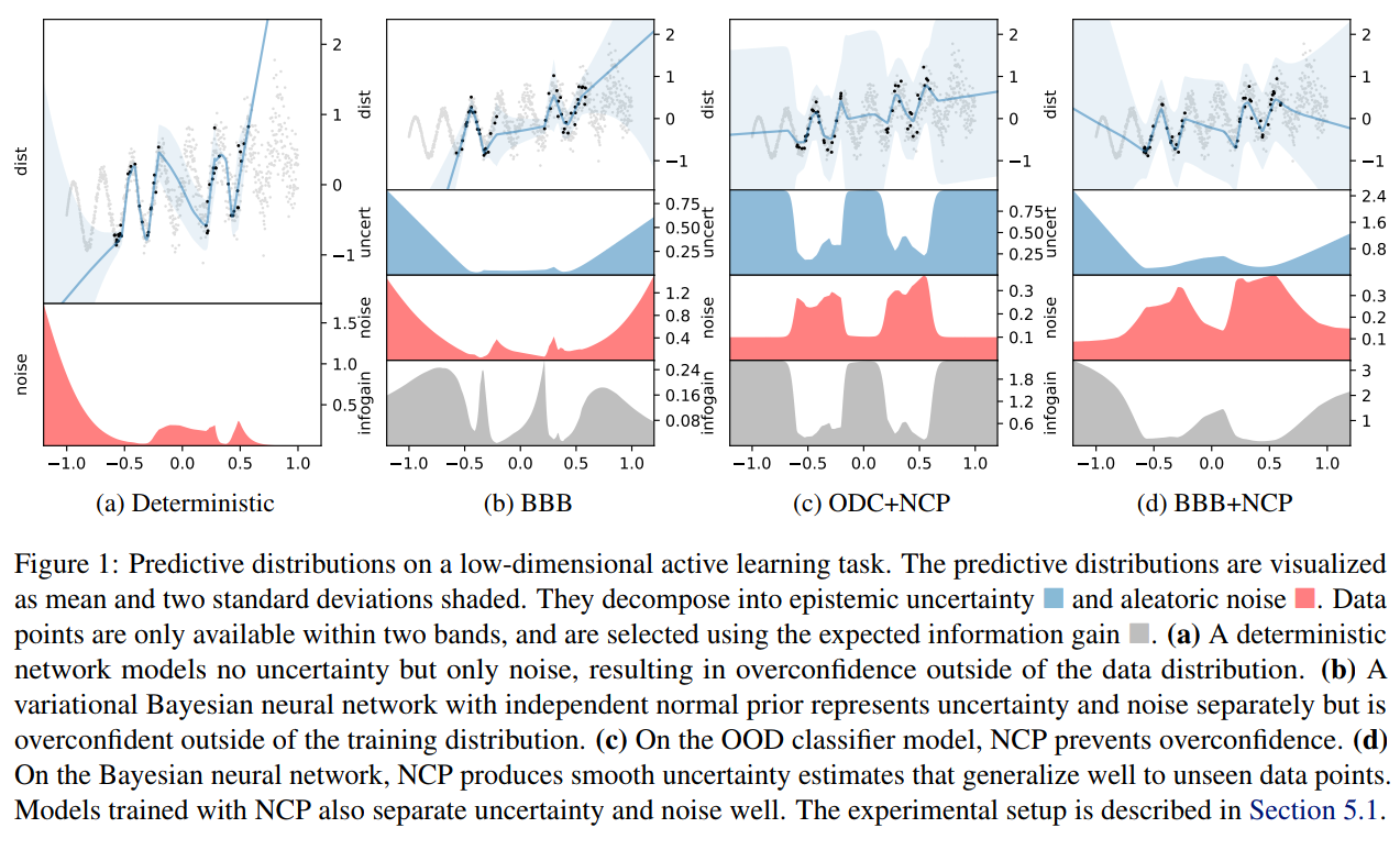
These are not the only methods
- Noise contrastive priors: https://arxiv.org/abs/1807.09289
Takeaway message on Bayesian Neural Networks
- They give a practical way to model epistemic uncertainties, aka unknowns unknows, aka errors on errors
- Be very careful when interpreting their output distributions, they are Bayesian posterior, yes, but under what priors?
- Having access to model uncertainties can be used for active sampling
Solution Notebook
Bonus Notebook Implementing a Normalizing Flow
Deep Probabilistic Learning
By eiffl
Deep Probabilistic Learning
Probabilistic Learning lecture at Advanced Euclid School, June 2022


