Introduction to Machine Learning
PHYS188/288: Bayesian Data Analysis And Machine Learning for Physical Sciences
Uroš Seljak
Delivered today by Francois Lanusse
Follow along at https://slides.com/eiffl/intro2ml/live
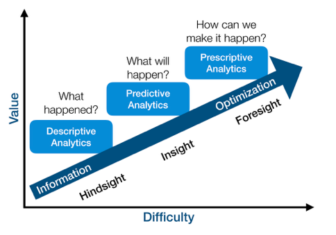
The different flavors of ML
From some input x, output can be:
- Summary z: unsupervised learning (descriptive, hindsight)
- Prediction y: supervised learning (predictive, insight)
- Action a to maximize reward r: reinforcement learning (prescriptive, foresight)
Value vs difficulty (although this view is subjective)
- Supervised learning: classification and regression
- Unsupervised learning: e.g. dimensionality reduction, clustering
Data Analysis vs Machine Learning
- In physical sciences we usually compare data to a physics based model to infer parameters of the model. This is often an analytic model as a function of physical parameters (e.g. linear regression). This is the Bayesian Data Analysis component of this course. We need likelihood and prior.
- In machine learning we usually do not have a model, all we have is data. If the data is labeled, we can also do inference on a new unlabeled data: we can learn that data with certain value of the label have certain properties, so that when we evaluate a new data we can assign the value of the label to it. This works both for regression (continuous values for labels) or classification (discrete label values).
-
Hybrid: Likelihood free inference (LFI), i.e. inference using ML methods. Instead of doing prior+likelihood analysis we make labeled synthetic data realizations using simulations, and use ML methods to infer the parameter values given the actual data realization. We pay the price of sampling noise, in that we may not have sufficient simulations for ML methods to learn the labels well.
- For very complicated, high dimensional problems, full Bayesian analysis may not be feasible and LFI can be an attractive alternative. We will be learning both approaches in this course.
Supervised Learning
Supervised Learning (SL)
- What is Supervised Learning?
- Answering a specific question: e.g. regression or classification
- We know the correct answer for part of the data
- Supervised learning is essentially interpolation
- General recipe:
- Frame the problem, collect the data
- Choose the SL algorithm
- Choose objective function (decide what to optimize)
- Train the algorithm, test (cross-validate)
Classes of problems: Regression

Basic Machine Learning Procedure
-
We have some data x and some labels y, such that Y=(x,y). We wish to find some model G(a) and some loss function C(Y, G(a)) that we wish to minimize such that the model explains the data Y.
- For instance:
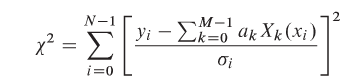
Y = (x, y)
G(a) = a_0 X_0(x_i) + a_1 X_1(x_i) + \ldots + a_{M-1} X_{M-1}(x_i)
C = \chi^2

x
y
f(x) = 2x, no noise
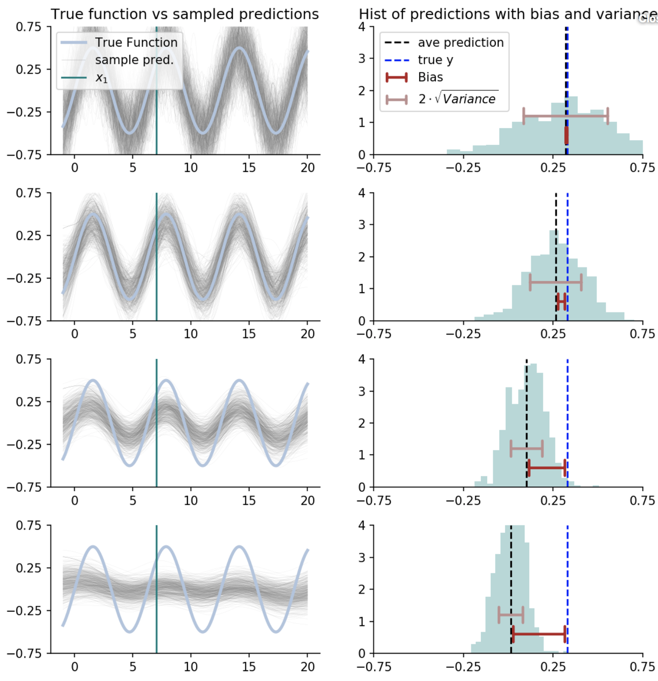
Over-fitting noise with too complex models (bias-variance trade-off)
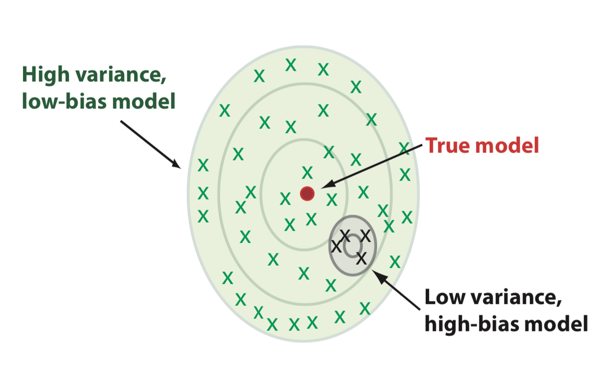
Bias-variance trade-off
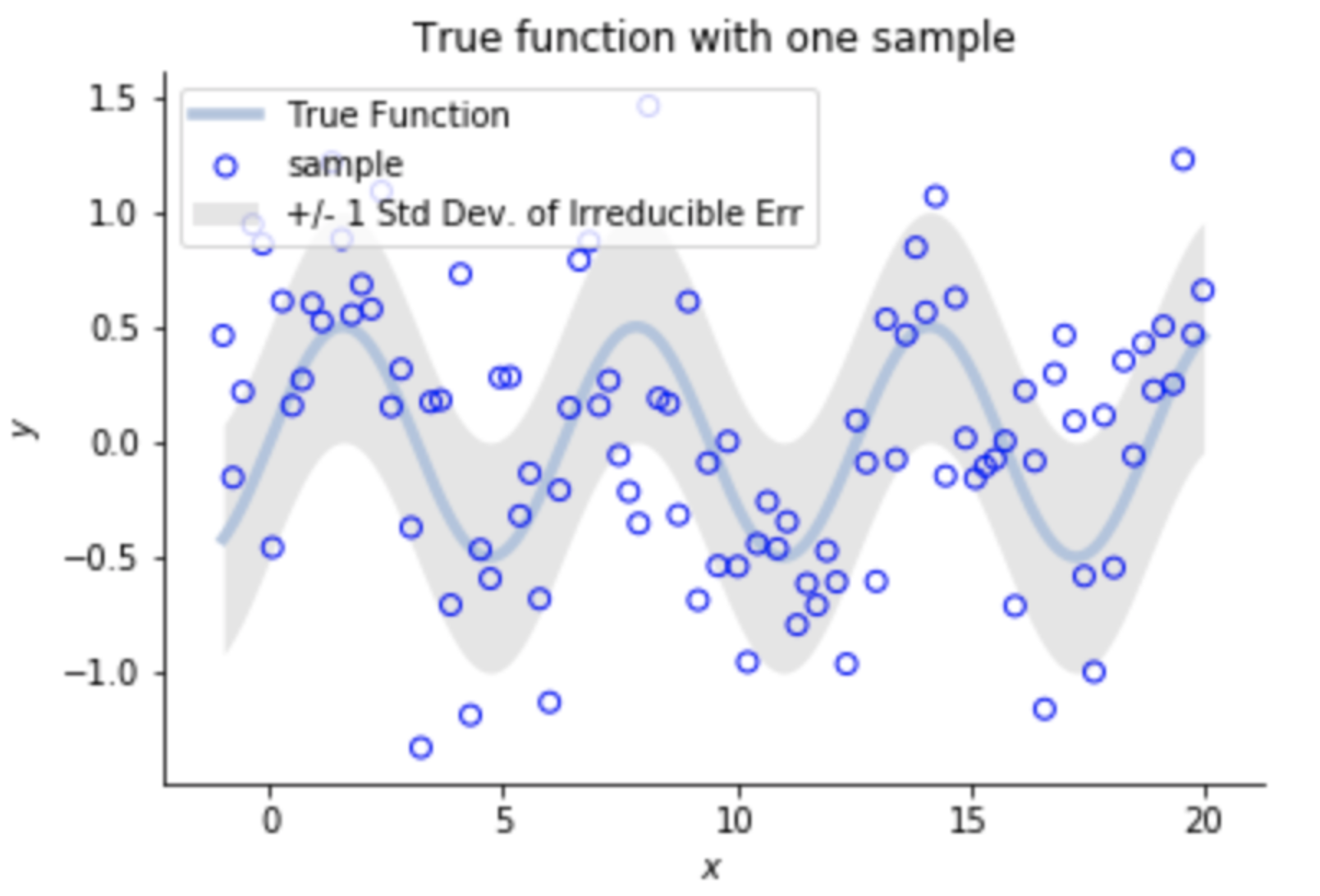
y = f(\bm{x}) + \epsilon
Let's model the data as:
Err = \mathbb{E}\left[ (y - f_{est}(\bm{x}))^2 \right]
= \mathbb{E} \left[ ( (f(\bm{x}) + \epsilon) - f_{est}(\bm{x}) )^2 \right]
= \mathbb{E} \left[ f(\bm{x} + \epsilon)^2 \right] - 2 \mathbb{E}[f_{est}(\bm{x}) (f(\bm{x}) + \epsilon)]
+ \mathbb{E} \left[ f_{est}(\bm{x})^2 \right]
= \sigma_\epsilon^2 + f(\bm{x})^2 - 2 f(\bm{x}) \mathbb{E} \left[ f_{est} (\bm{x}) \right] + \mathbb{E}\left[ f_{est}(\bm{x})^2 \right]\\
+ \underbrace{\mathbb{E}\left[ f_{est}(\bm{x}) \right]^2 - \mathbb{E}\left[f_{est}(\bm{x}) \right]^2}_{=0}
= \underbrace{\sigma_\epsilon^2} + \underbrace{\left( \mathbb{E}[f_{est}(\bm{x})] - f(\bm{x})\right)^2} + \underbrace{\mathbb{E}\left[ \left( f_{est}(\bm{x}) - \mathbb{E}[f_{est}(\bm{x})] \right)^2\right]}
Irreducible Error
Bias²
Variance
How do we find the right balance?
-
In ML we divide data into training data Y_train (e.g. 90%) and test data Y_test (e.g. 10%)
-
We fit model to the training data: the value of the minimum loss function at a_min is called:
in-sample error E_in=C(Y_train,g(a_min)) -
We test the results on test data, getting:
out of sample error E_out=C(Y_test,g(a_min)) > E_in -
This is called cross-validation technique
-
If we have different models then test data are called validation data while test data are used to test different models, each trained on training data (3 way split, e.g. 60%, 30%, 10%)
-
Statistical learning theory
- We have data and we can change the number of data points
- We have models and we can change complexity (number of model parameters in simple versions)
- Trade-off at fixed model complexity:
- Small data size suffers from a large variance (we are overfitting noise)
- Large data size suffers from model bias
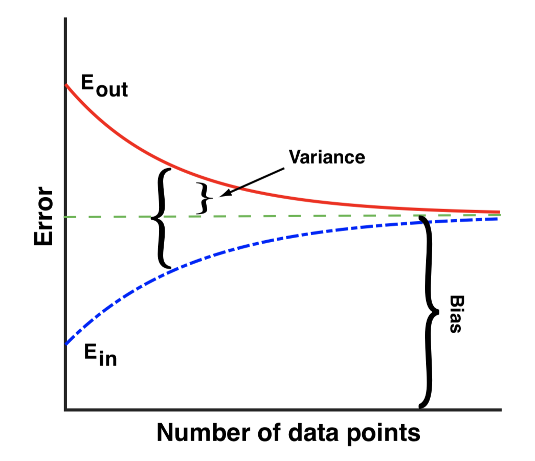
- Variance quantified by E_in vs E_out
- E_in and E_out approach bias for large data
- To reduce bias increase complexity
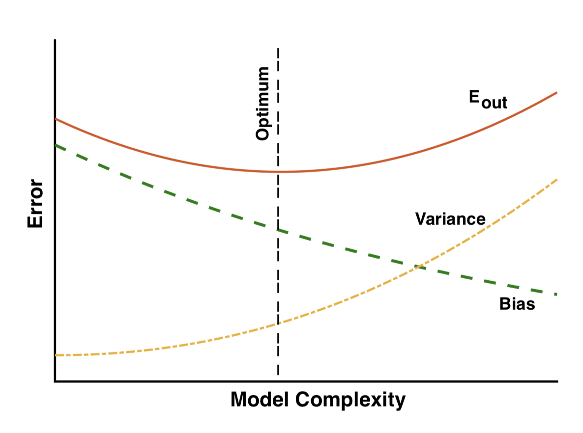
Bias-variance trade-off vs complexity
- Low complexity: large bias
- Large complexity: large variance
- Optimum when the two are balanced
- Complexity can be controlled by regularization (we will discuss it further)
Data Analysis vs ML
- Data analysis: fitting existing data to a physics based model to obtain model parameters y. Parameters are fixed: we know physics up to parameter values. Parameter posteriors are the goal.
- ML: use model derived from existing data to predict regression or classification parameters y for new data.
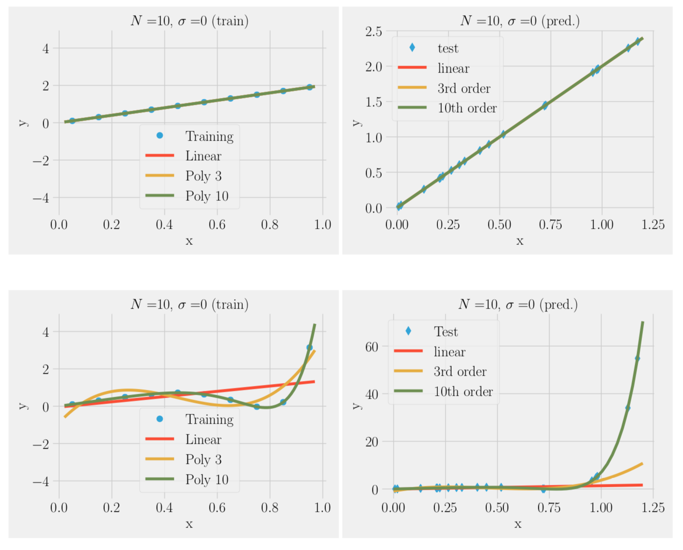
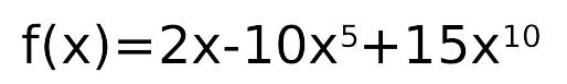
- Example: polynomial regression. This will be HW 4 problem
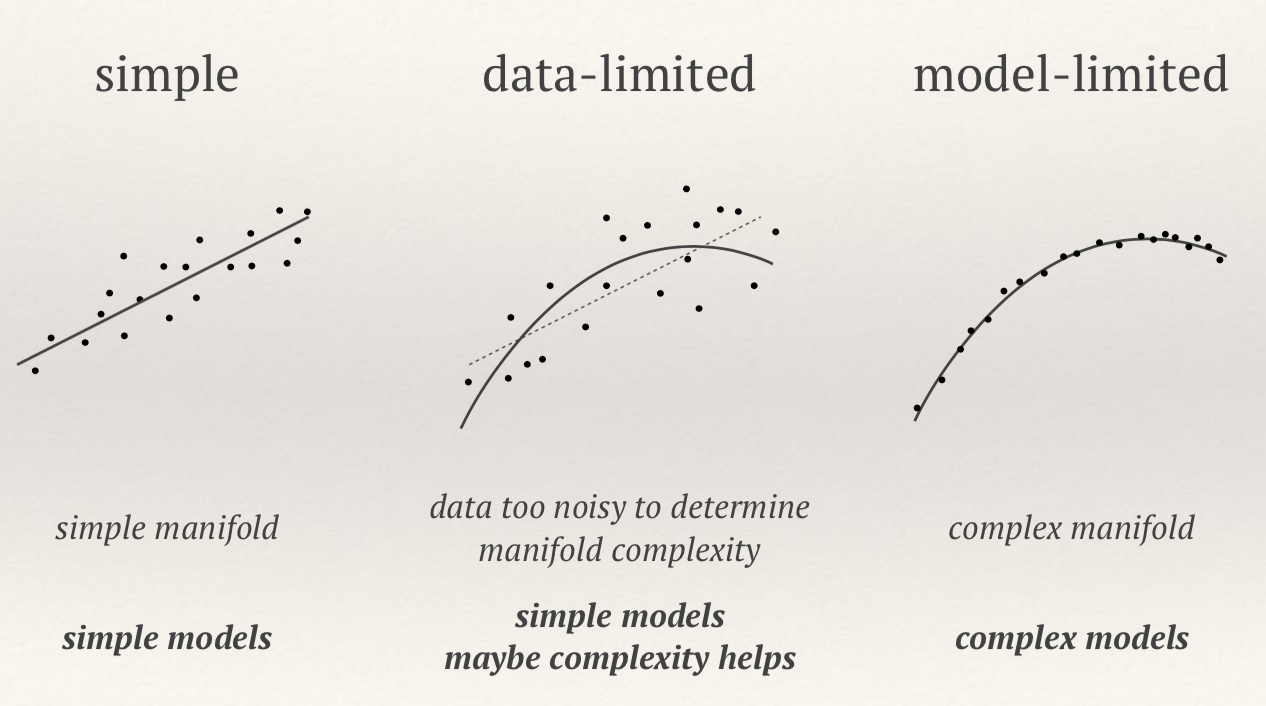
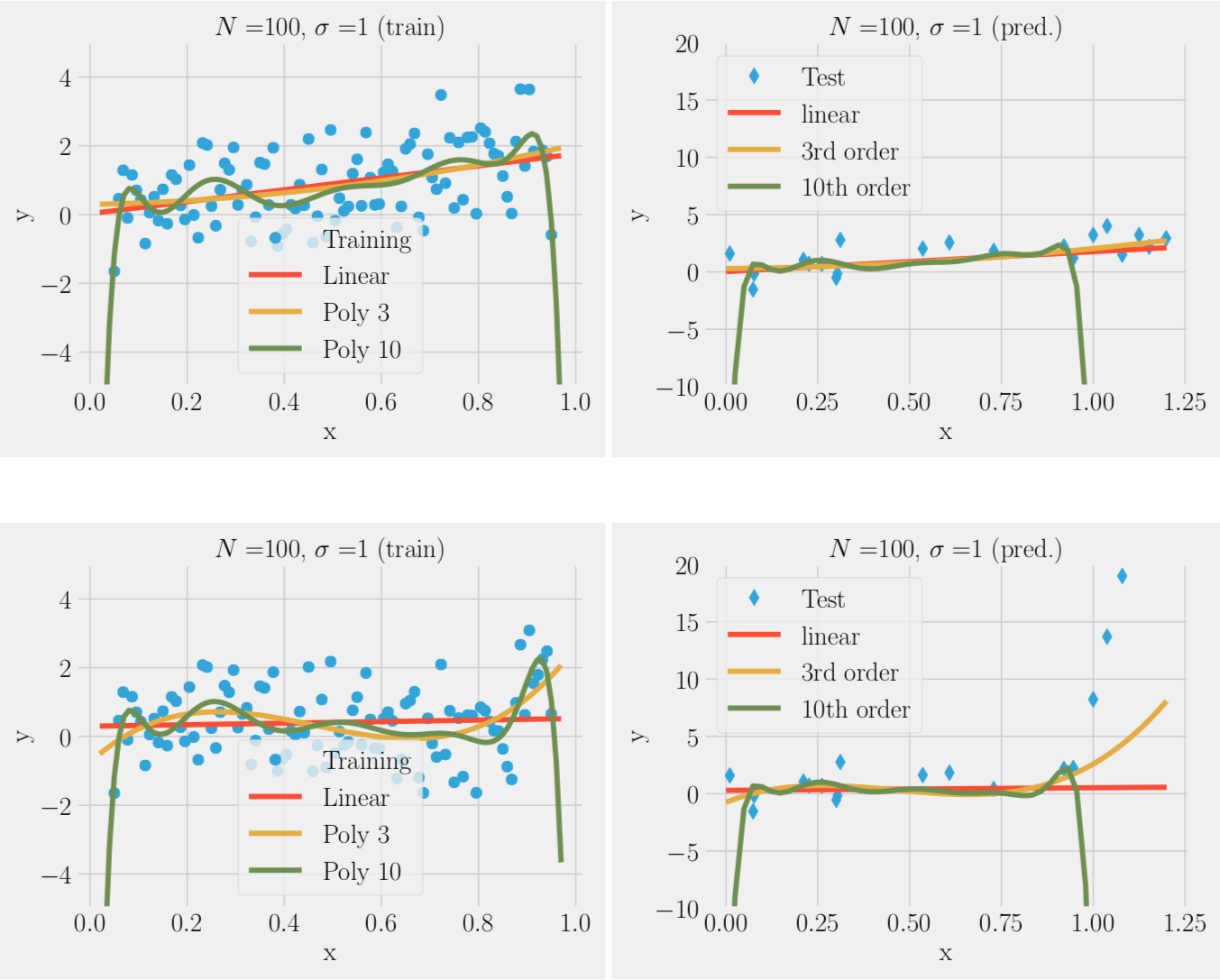
We can fit the training data to a simple model or complex model:
- In the absence of noise complex model (many parameters ) always better
- In the presence of noise complex model often worse
- Note that parameters a have no meaning on their own, just means to reach the goal of predicting y. The art of ML is to choose the best basis for this interpolation
Another example: k-nearest neighbors
How predictions change as we average over more nearest neighbours?
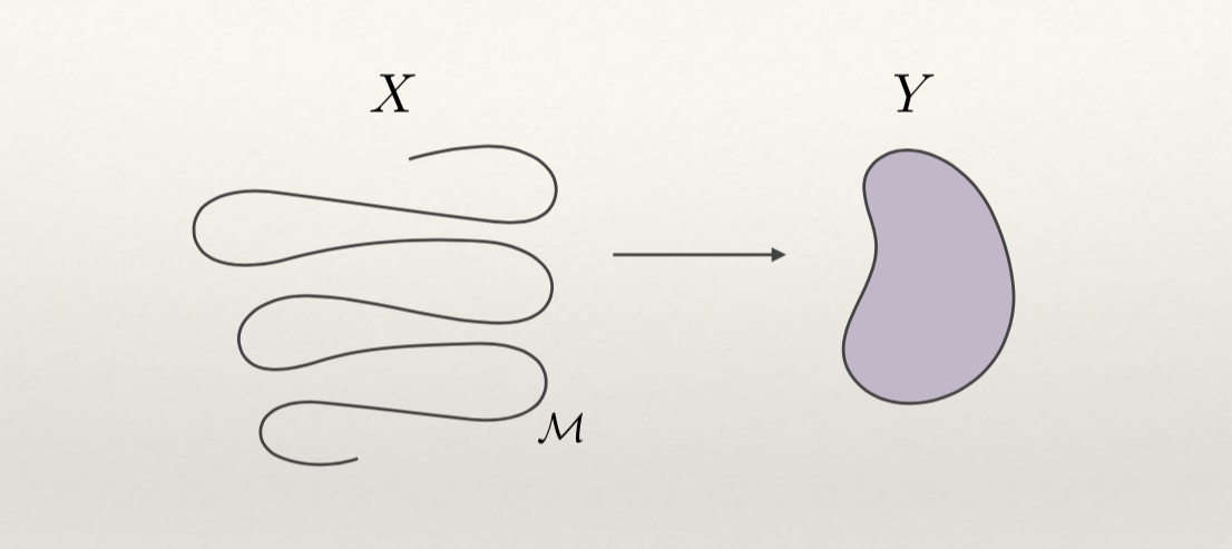
Representational power
-
We are learning a manifold M
-
To learn complex manifolds we need high representational power
-
We need a universal approximator with good generalization properties (from in-sample to out of sample, i.e. not over-fitting)
-
This is where neural networks excel: they can fit anything (literally, including pure noise), yet can also generalize
Unsupervised Learning
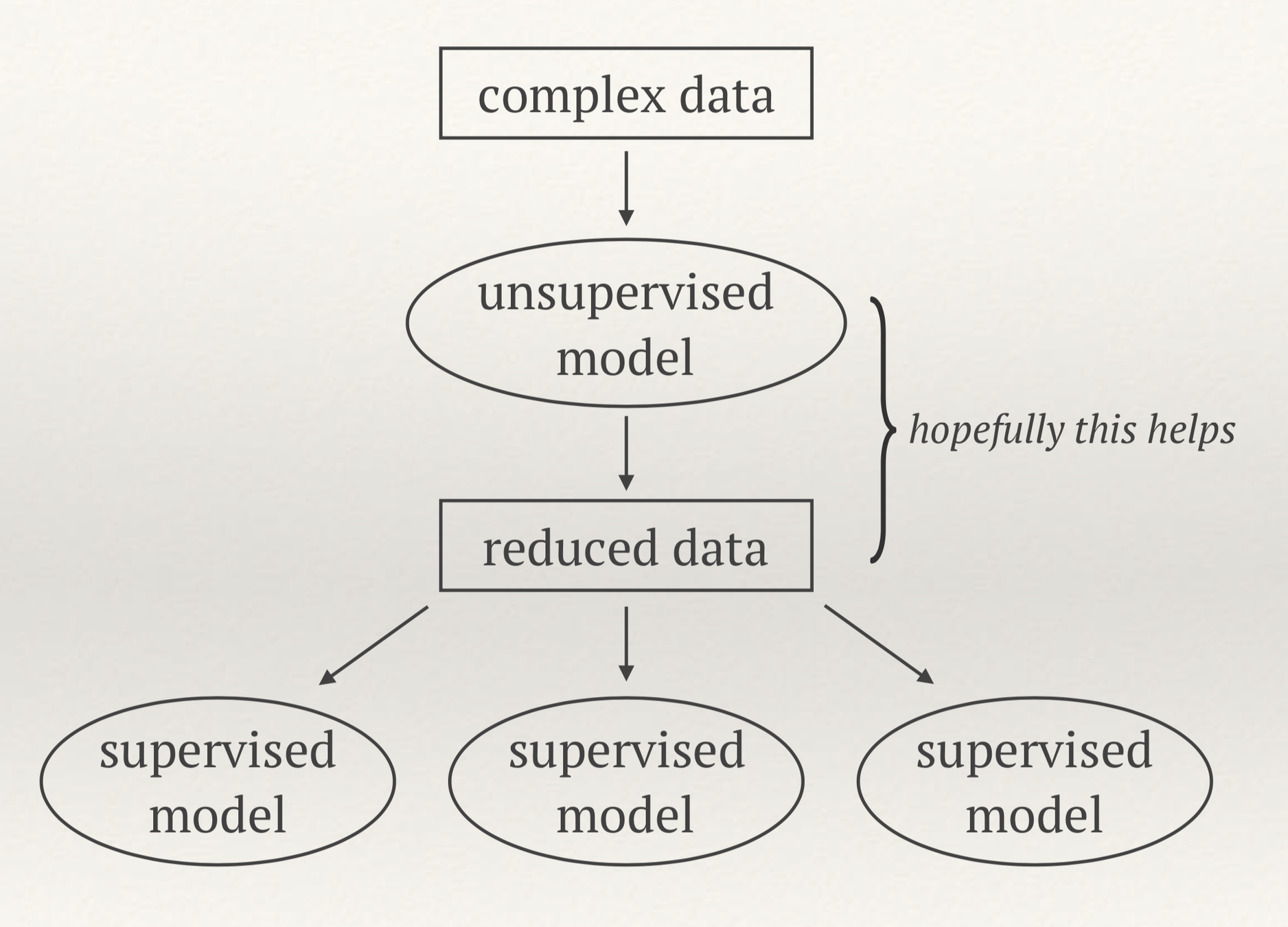
Unsupervised Machine Learning
- Discovering structure in unlabeled data
- Examples: clustering, dimensionality reduction
- The promise: easier to do regression, classification
- Easier visualization
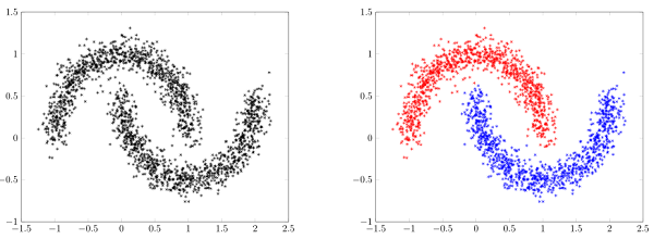
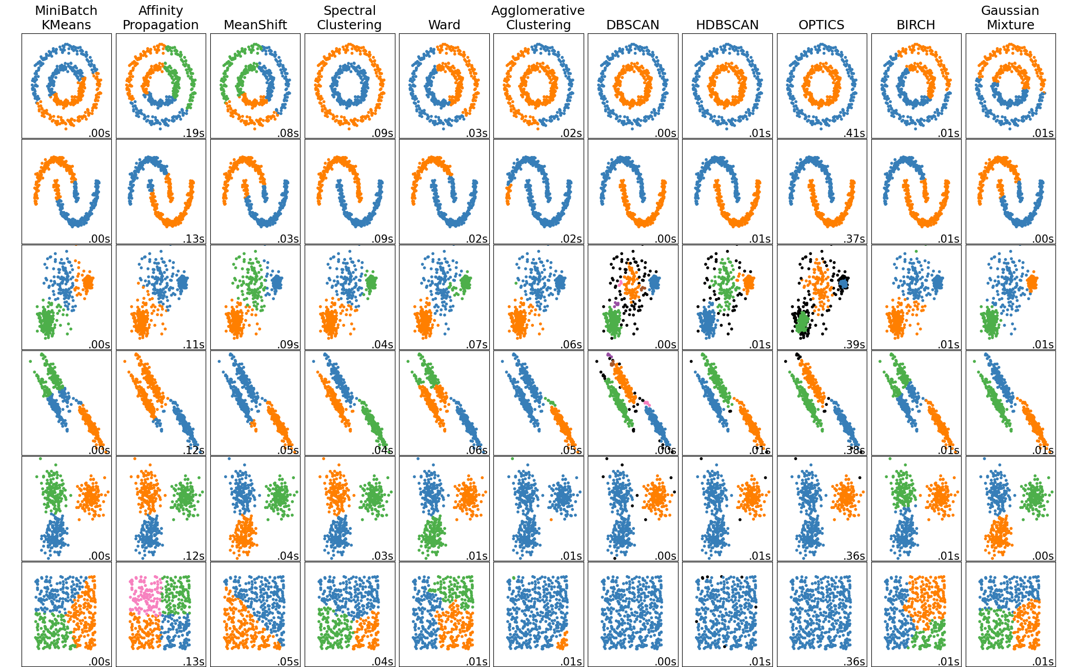
Clustering algorithms
- For unsupervised learning (no labels available) we want to identify similarities in the data
- Clustering algorithms can regroup data points based on their proximity
- Main big families of clustering algorithms:
- Centroid-based clustering (e.g. k-means)
- Distribution-based clustering (e.g. Gaussian mixture)
- Density-based clustering (e.g. DBSCAN)
- We will look at k-means and Gaussian mixture model later
- They both usually require choosing the
number of clusters
- They both usually require choosing the
- HW 3: UMAP + clustering

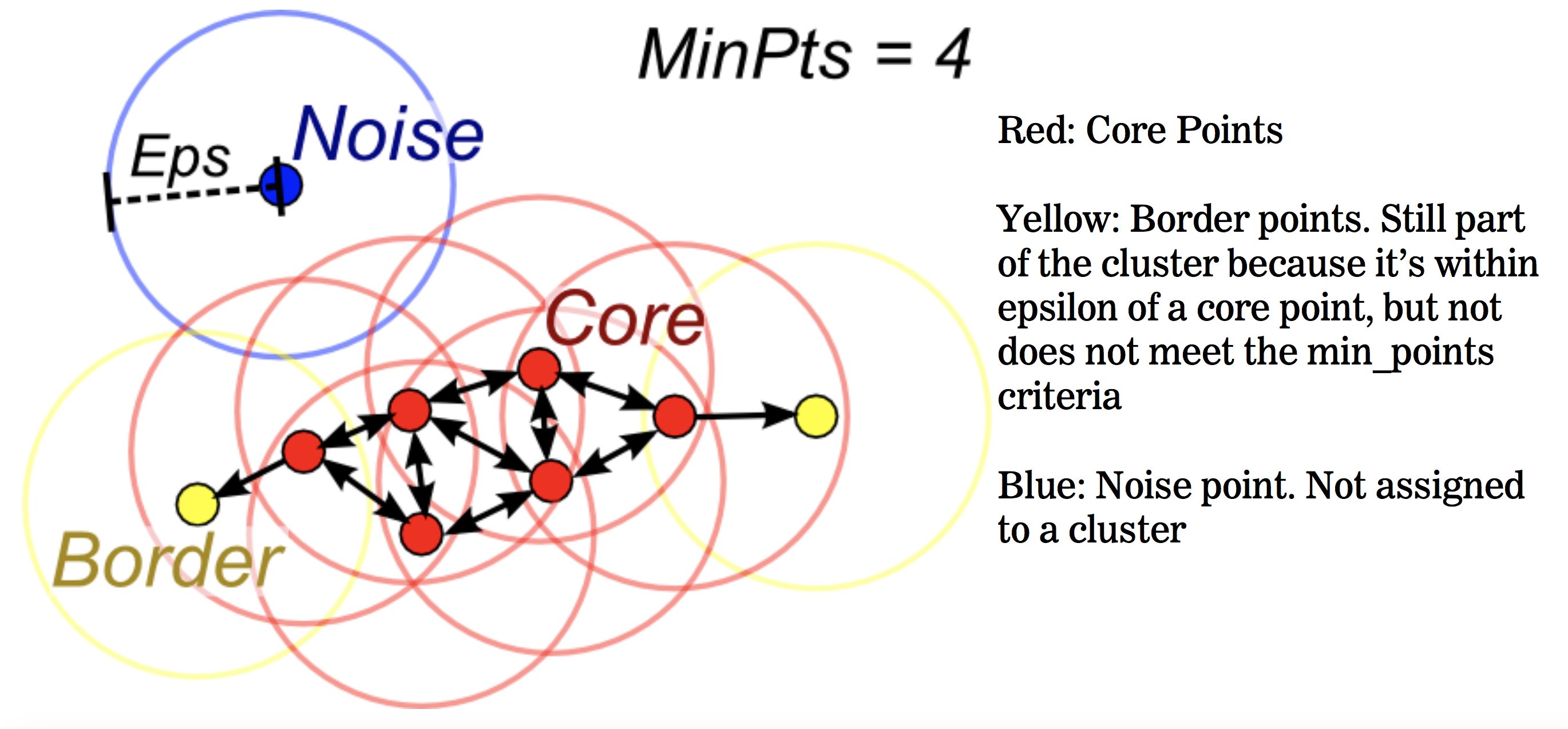
DBSCAN
Density-based spatial clustering of applications with noise
Main idea:
- Estimate the density
- Apply a density threshold
- Identify connected components
How do we measure this density?
- p is a core point if:
at least MinPts are within distance Eps - p is a border point if:
fewer than MinPts are within distance Eps - p is a noise point if:
no points within distance Eps
Algorithm outline:
- Find the Eps neighboors of all points, identify core points
- Identify the connected components for the core points graph
- Assign each border point to a component if one is reachable, otherwise assign to noise
Many more clustering algorithms
Why do we need more than clustering ?
- Usually doesn't work well in high number of dimensions
- We need a notion of distance for doing clustering
- In high dimensions, the curse of dimensionality reduces the differences in distances between pairs of points

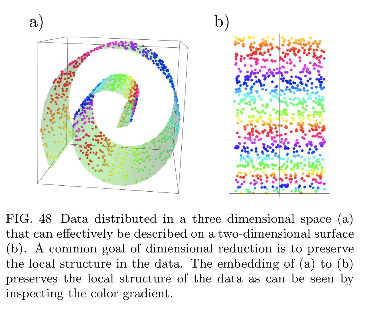
Dimensionality Reduction
- PCA (lecture 4), ICA (lecture 5)
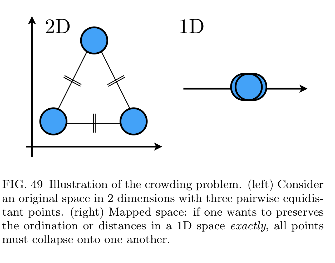
- Manifold projection: want to reduce it preserving pairwise distance between data points (e.g. t-SNE, ISOMAP, UMAP).
- If reduced too much we get crowding problem
t-SNE
t-Distributed Stochastic Neighbor Embedding
What do we want for good dimensionality reduction?
- Lowers dimension
- Preserves notion of neighborhood
- We need define a probability of neighborhood in high dimensionality space


- Probability of neighborhood in low-dimensionality space:
- Distance between these distributions
\text{KL}(P||Q) = \sum_i P_i \log \left( \frac{P_i}{Q_i} \right)
= \sum_i P_i \log \left( P_i \right) - \sum_i P_i \log \left( Q_i \right)
= - H(P) + H(P, Q)
\frac{\partial C}{\partial y_{i}} = \frac{\partial \text{ KL}(P \vert \vert Q)}{\partial y_{i}}
= 4\sum_{j}(p_{ij}-q_{ij})(y_i-y_j)(1+||y_i-y_j||^2)^{-1}
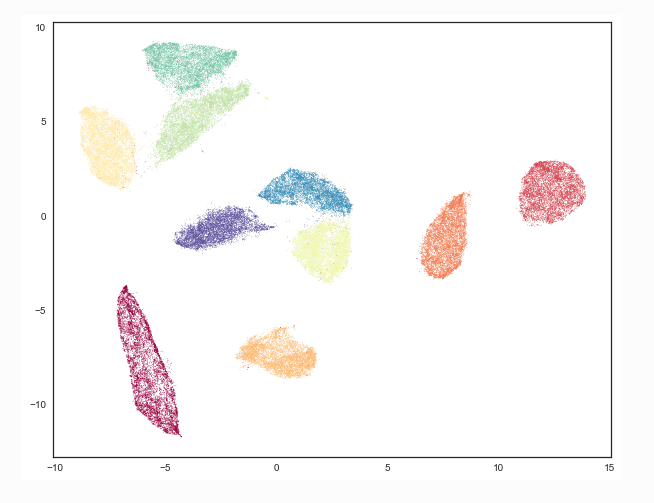
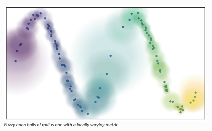
UMAP: Uniform Manifold Approximation and Projection for Dimension Reduction
- Tries to connect nearby points using locally varying metric
- Best on the market at the moment
- You will try it in HW3
- Example MNIST digits separate in 2d UMAP plane
Literature
- Numerical Recipes, Press et al., Chapter 15
(http://apps.nrbook.com/c/index.html) - Bayesian Data Analysis, Gelman et al. , Chapter 1-4
- https://umap-learn.readthedocs.io/en/latest/how_umap_works.html
- A high bias, low variance introduction to machine learning for physicists, https://arxiv.org/pdf/1803.08823.pdf (pictures on slides taken from this review)
Introduction to Machine Learning
By eiffl
Introduction to Machine Learning
Bayesian Data Analysis And Machine Learning for Physical Sciences


