Recurrent Inference Machines for Inverse Problems
Berkeley Statistics and Machine Learning Forum
From Compressed Sensing to Deep Learning
Inverse Problems
y = \mathbf{A} x + n
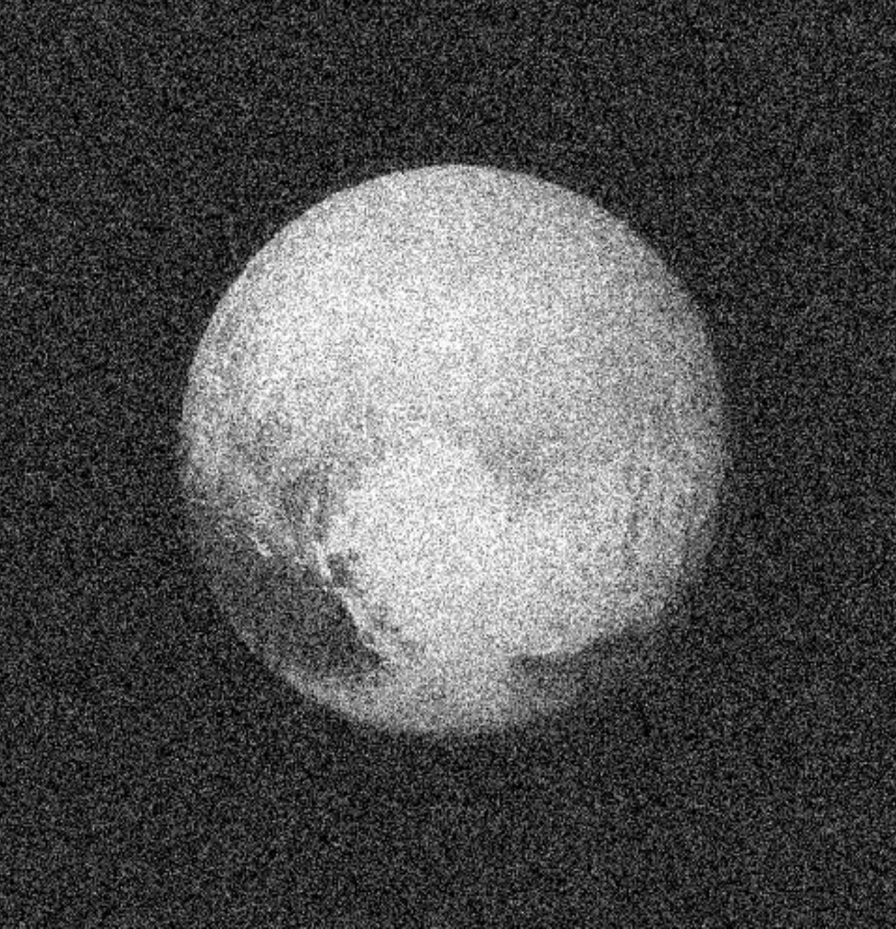
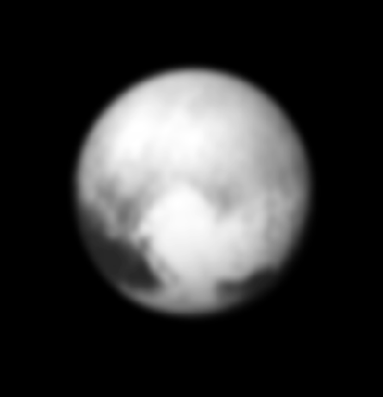
Denoising
Deconvolution
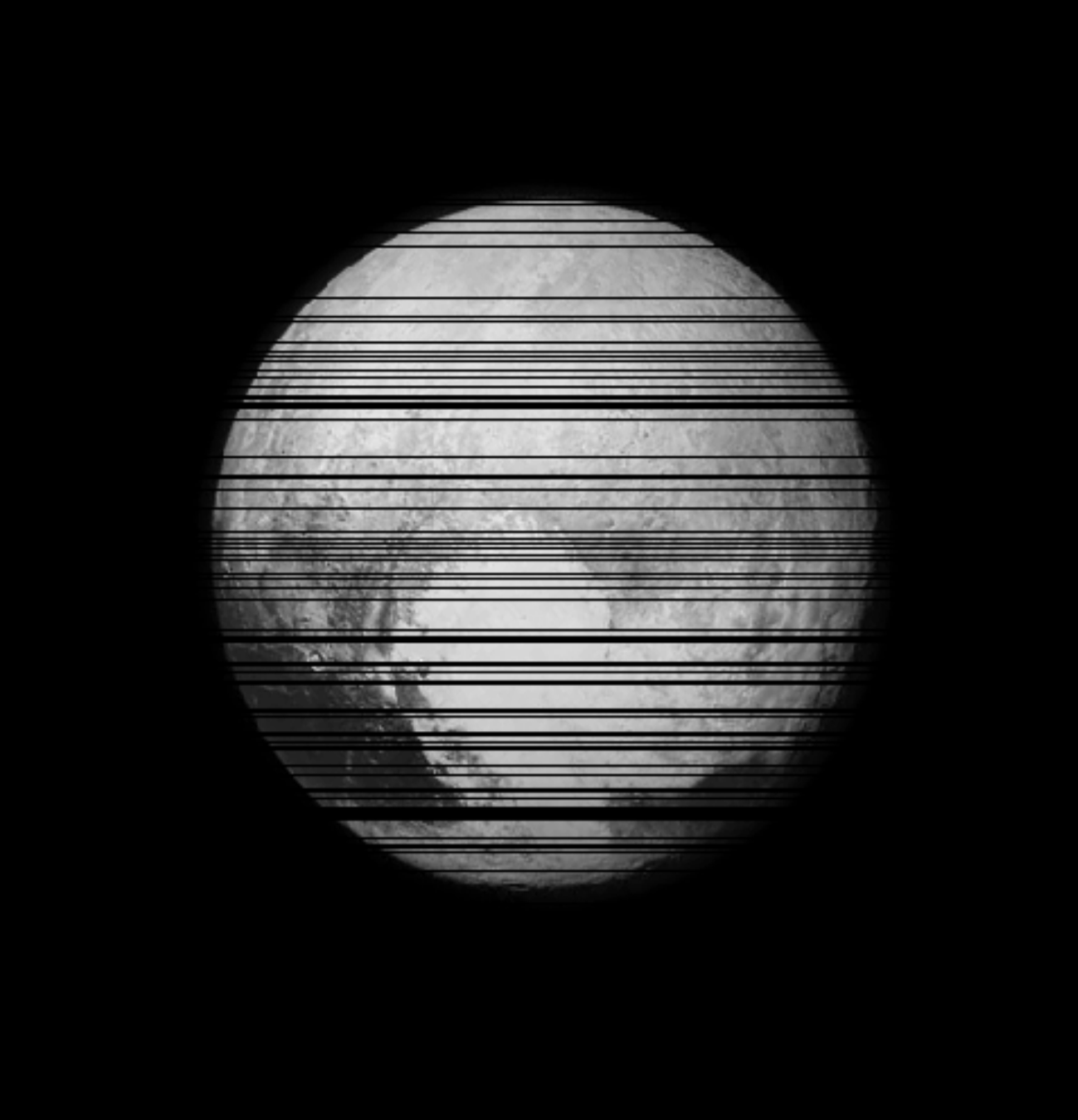
Inpainting
The Bayesian Approach
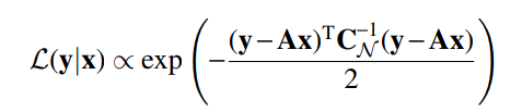
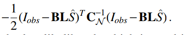
- p(y | x) is the likelihood function, contains the physical modeling of the problem:
-
p(x) is the prior, contains our assumptions about the solution
- Typically, people look for a point estimate of the solution, the Maximum A Posteriori solution:
p(x | y) \propto p(y | x) p(x)
p(y | x) = \mathcal{N}( \mathbf{A} x, \sigma^2)
\hat{x}_{MAP} = \argmax_x \log p(y |x) + \log p(x)
Where does my prior come from ?
\log p(x) = \parallel \mathbf{W} x \parallel_1
\log p(x) = \parallel x \parallel_\Sigma^2
\log p(x) = \parallel \nabla x \parallel_1
Wavelet Sparsity
Total Variation
Gaussian
Classical Image Priors
Image Restauration by Convex Optimization
- Simple differentiable priors: gradient descent
- Non differentiable priors: proximal algorithms
x_{t+1} = x_t + \lambda_t ( \nabla_x \log p(y | x_t) + \nabla_x \log p(x_t) )
\tilde{x}_{t+1} = x_t + \lambda_t ( \nabla_x p(y | x_t) )\\
x_{t+1} = \mathrm{prox}_{\lambda_t p(x)} (\tilde{x}_{t+1})
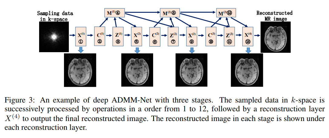
Unrolling Inference
Interpreting optimization algorithms as Deep Neural Networks
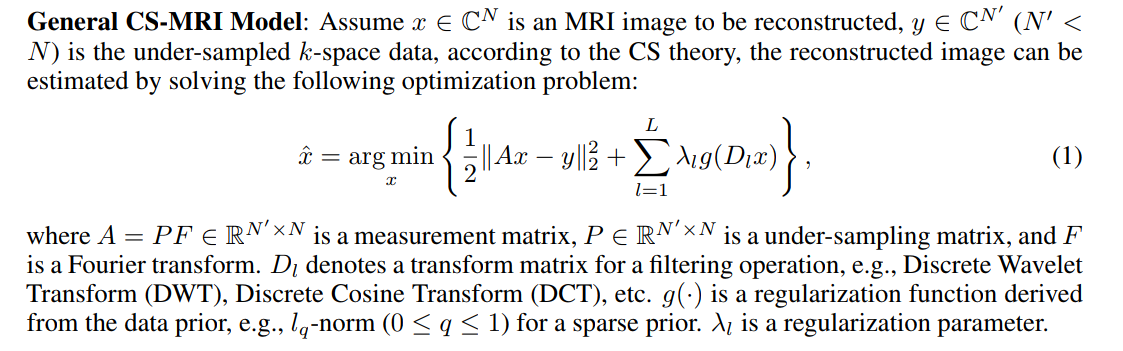
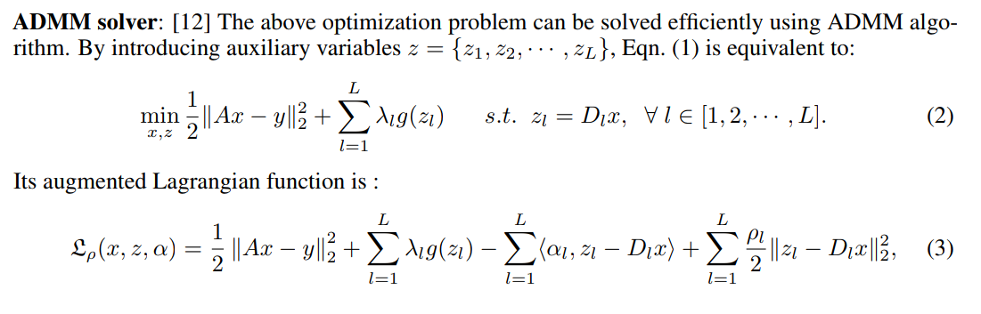
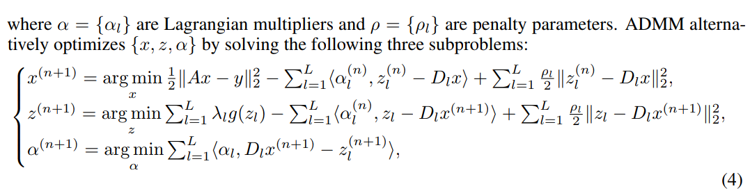
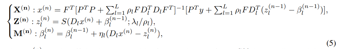
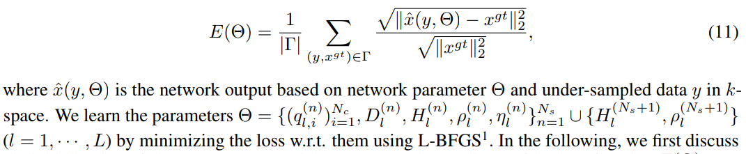
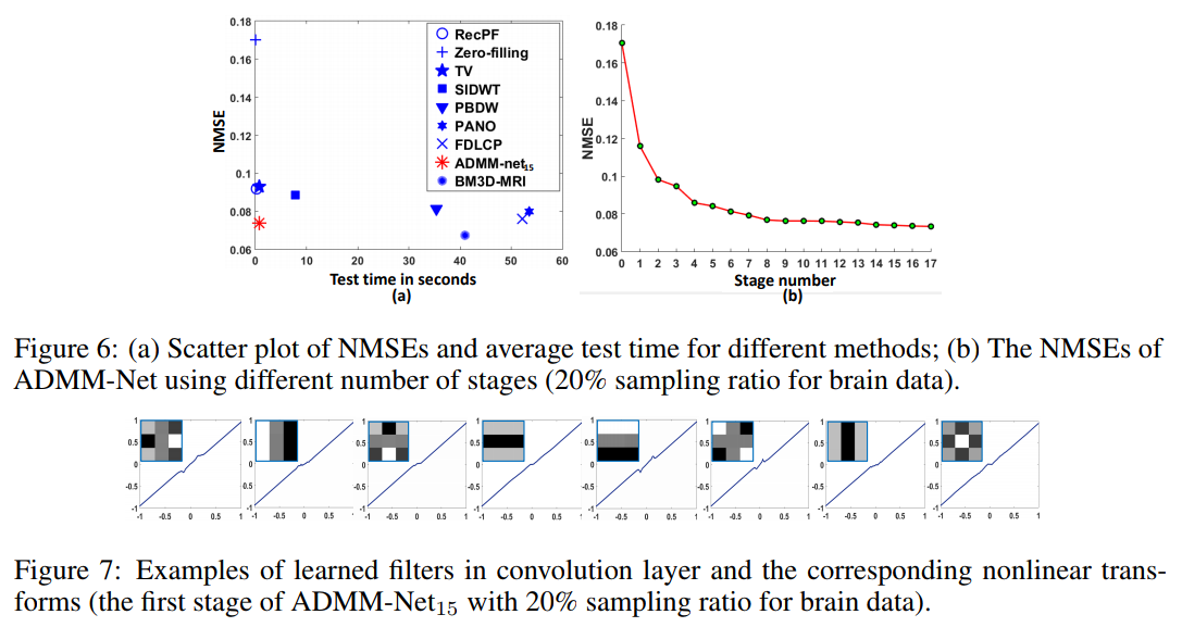
Example in MRI: Deep ADMM-Net for Compressive Sensing MRI
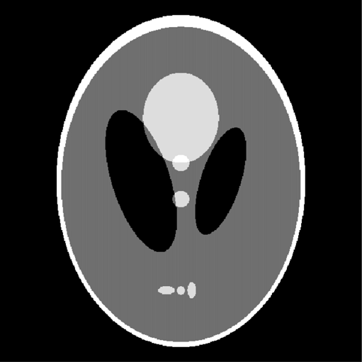
Compressive Sensing for MRI
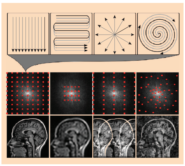
Credit: Lustig et al. 2008
Solving by ADMM

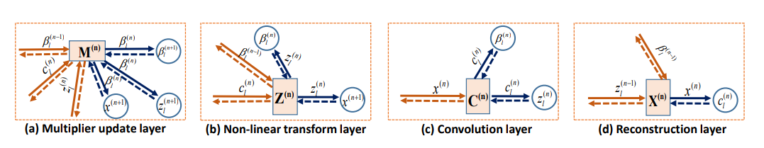
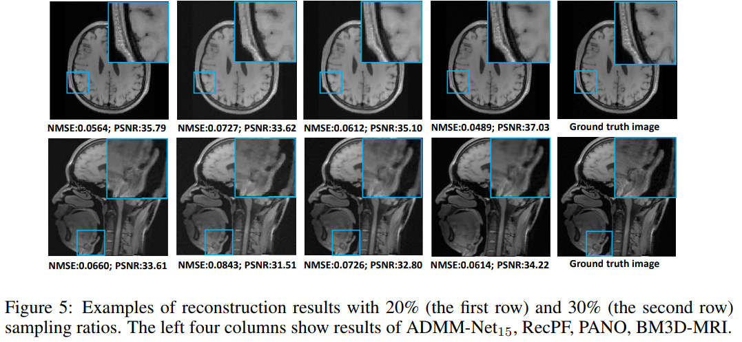
Advantages of the approach
- Automatically tune optimization parameters for faster convergence
- Automatically learns optimal representation dictionary
- Automatically learns optimal proximal operators
This is great, but can we do better?
Learning the Inference
Recurrent Inference Machines for Solving Inverse Problems
Putzky & Welling, 2017
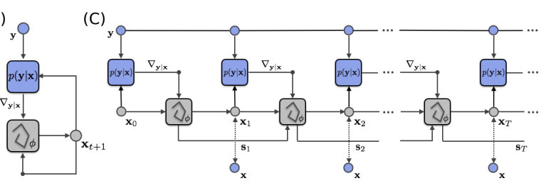
Reinterpreting MAP inference as a RNN
x_{t+1} = x_t + \lambda_t ( \nabla_x \log p(y | x_t) + \nabla_x \log p(x_t) )
x_{t+1} = x_t + g_\phi(\nabla_x p(y | x_t), x_t )
Why not write this iteration as:
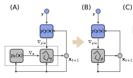
- Update strategy and step size become implicit
- Prior becomes implicit
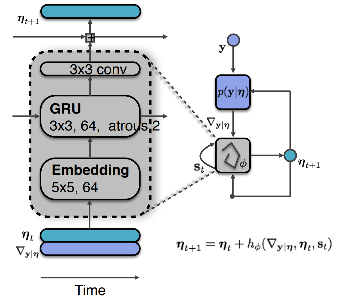
\mathcal{L^{(\phi)}} = \sum_{t=1}^T w_t \mathcal{L(x_t^{(\phi)}, x)}
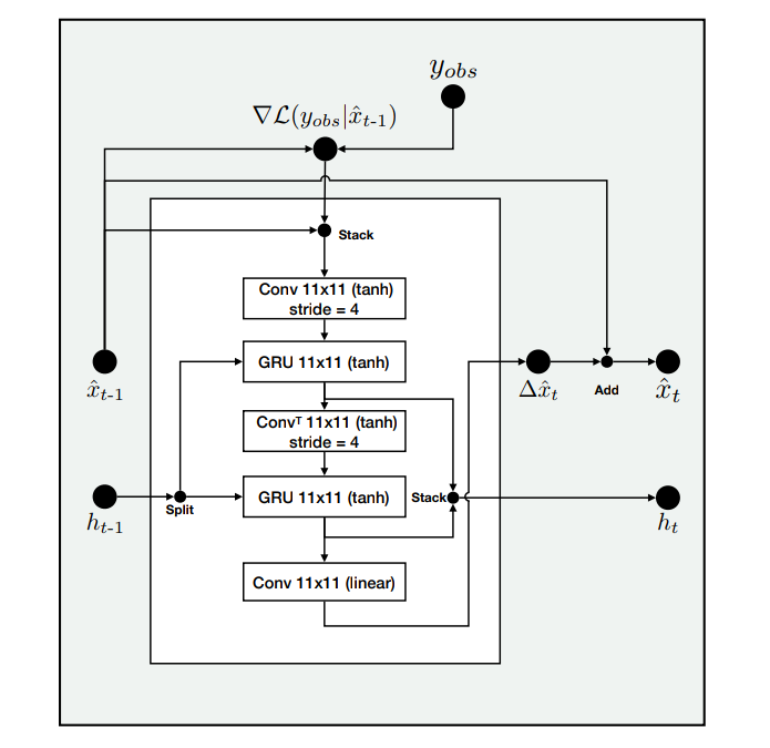
To match the RNN framework, an additional variable s is introduced to store an optimization memory state.
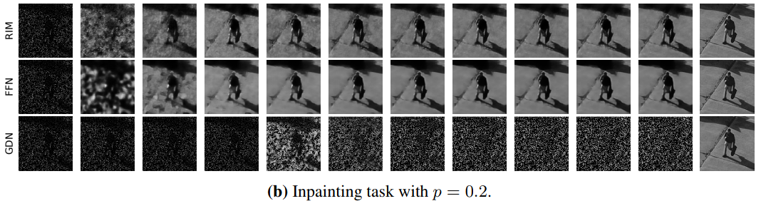
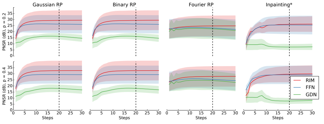
We trained three models on these tasks: (1) a Recurrent Inference Machine (RIM) as described in 2, (2) a gradient-descent network (GDN) which does not use the current estimate as an input (compare Andrychowicz et al. [15]), and (3) a feed-forward network (FFN) which uses the same inputs as the RIM but where we replaced the GRU unit with a ReLu layer in order to remove hidden state dependence.
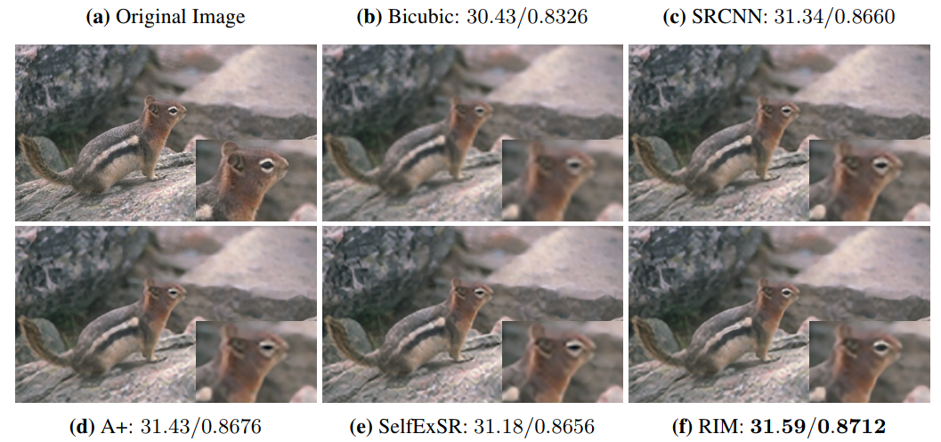
Super-resolution example with factor 3
Applications in the Wild 1/2
Recurrent Inference Machines
for Accelerated MRI Reconstruction
Lønning et al. 2018
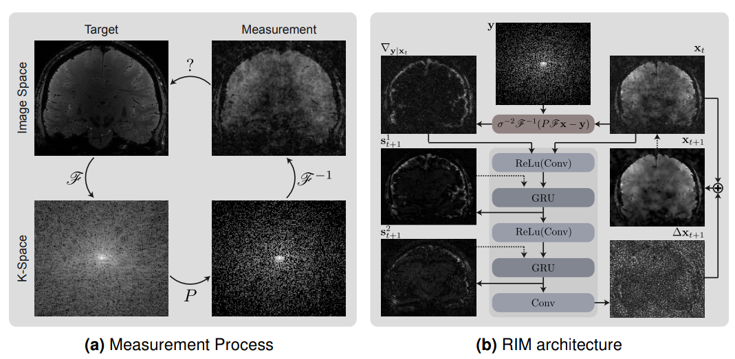

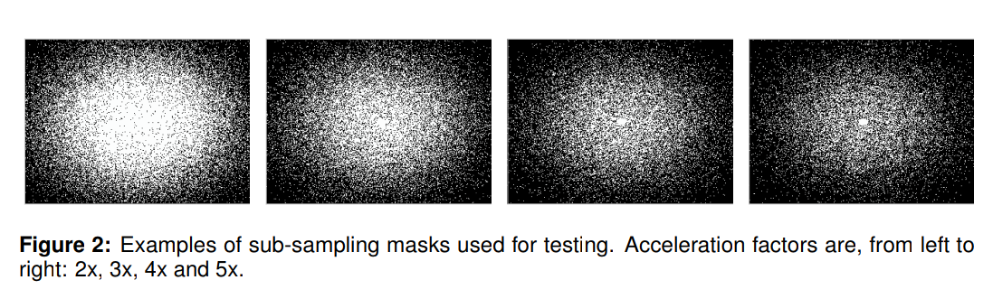
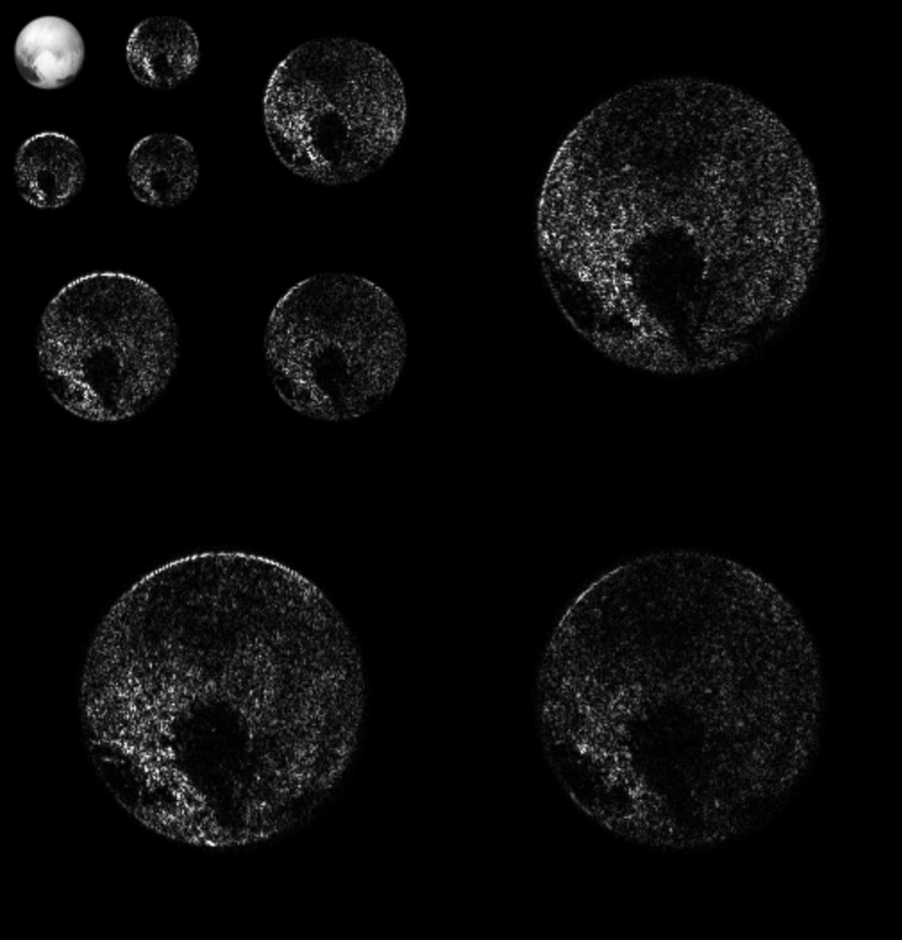
All models in this paper were trained on acceleration factors that were randomly sampled from the uniform distribution U (1.5, 5.2). Sub-sampling patterns were then generated using a Gaussian distribution.
Applications in the wild 2/2
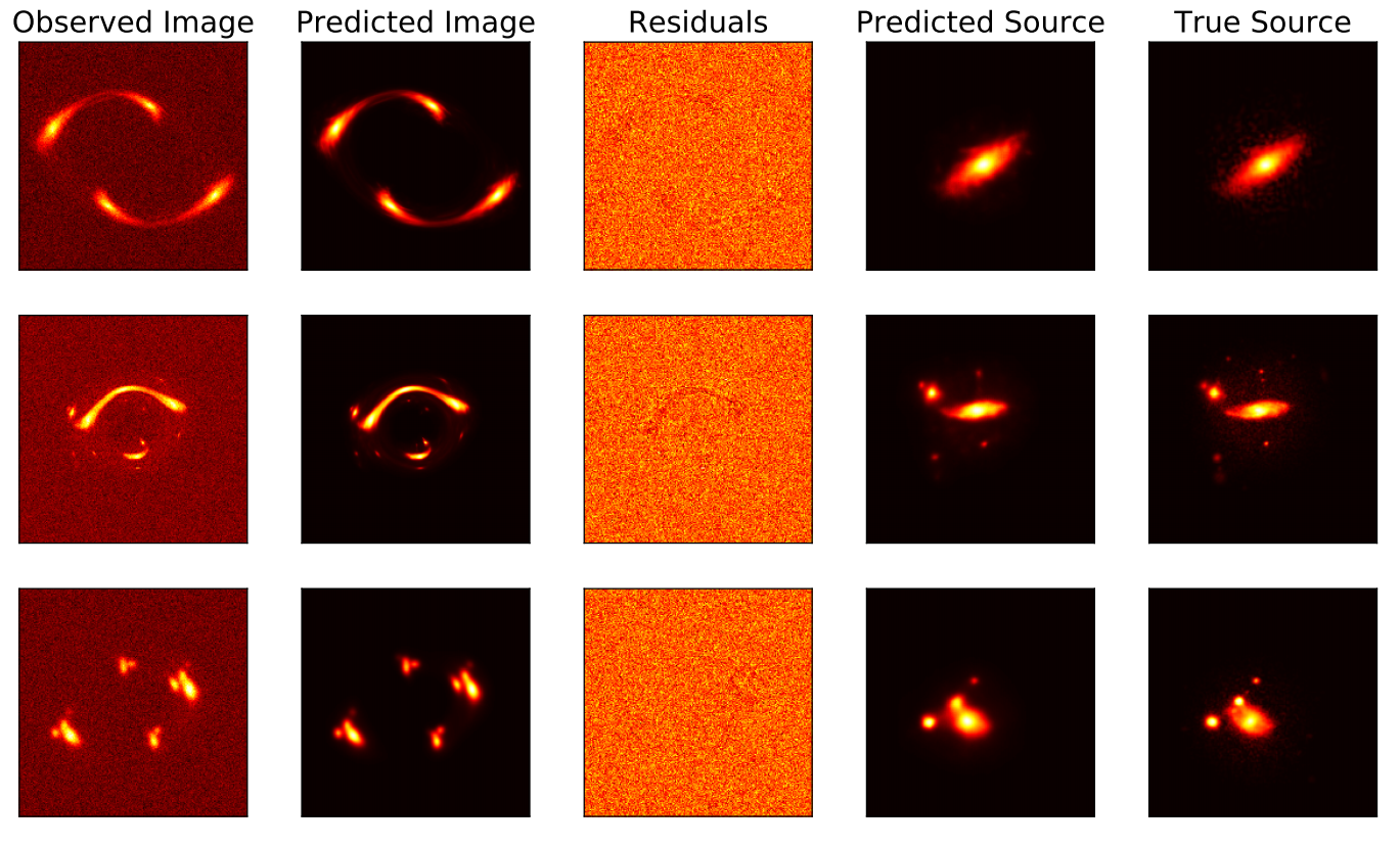
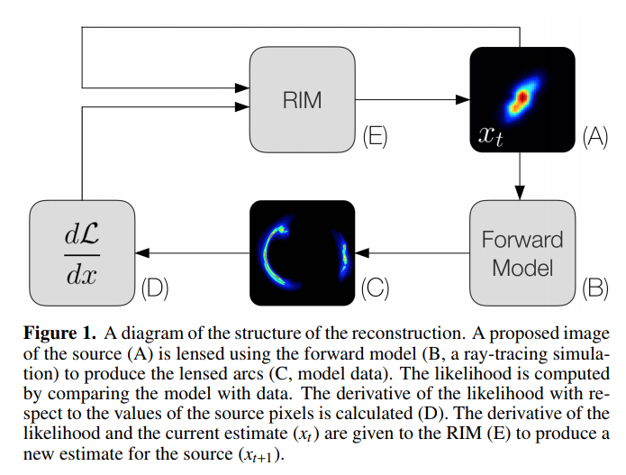
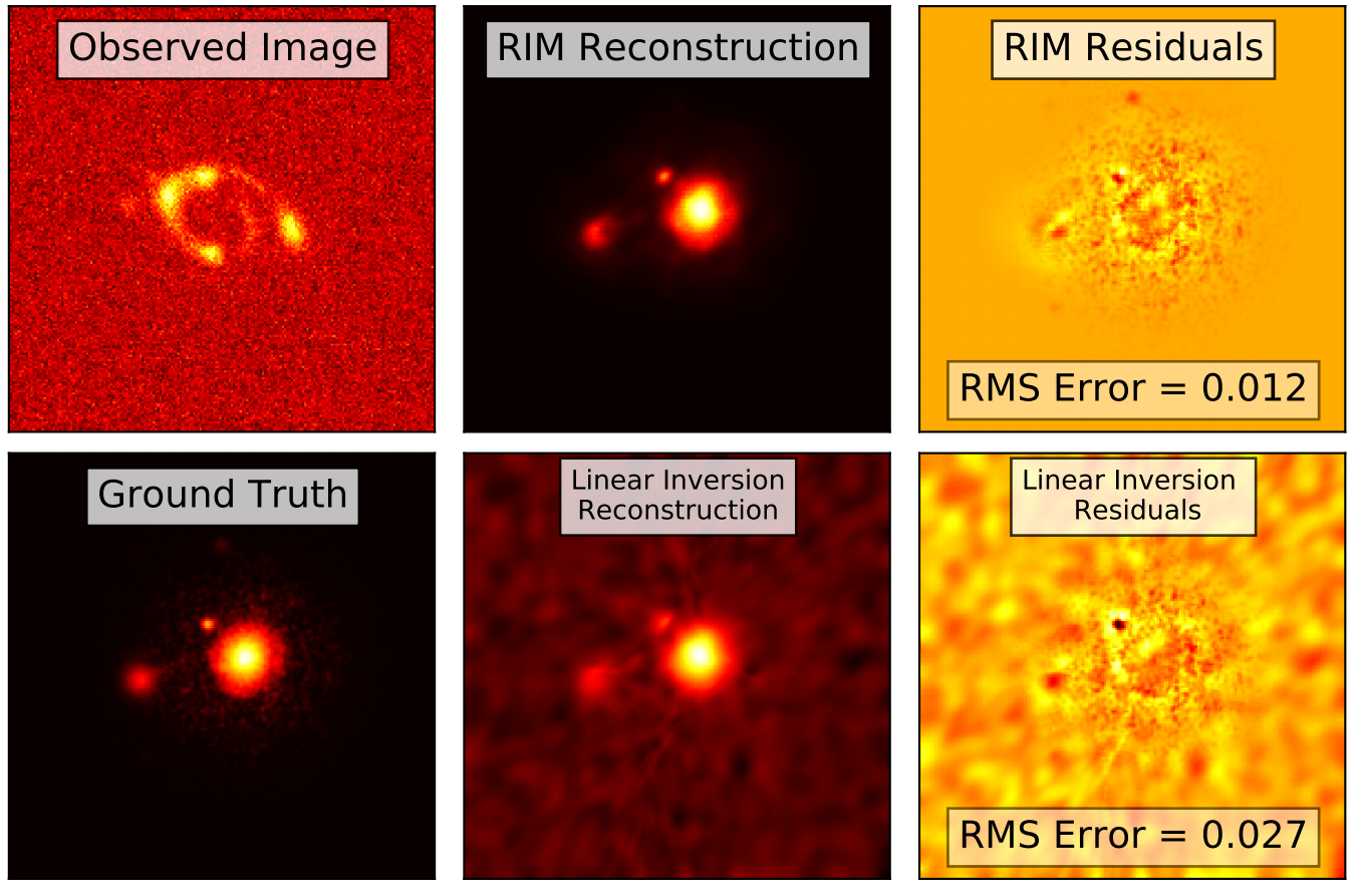
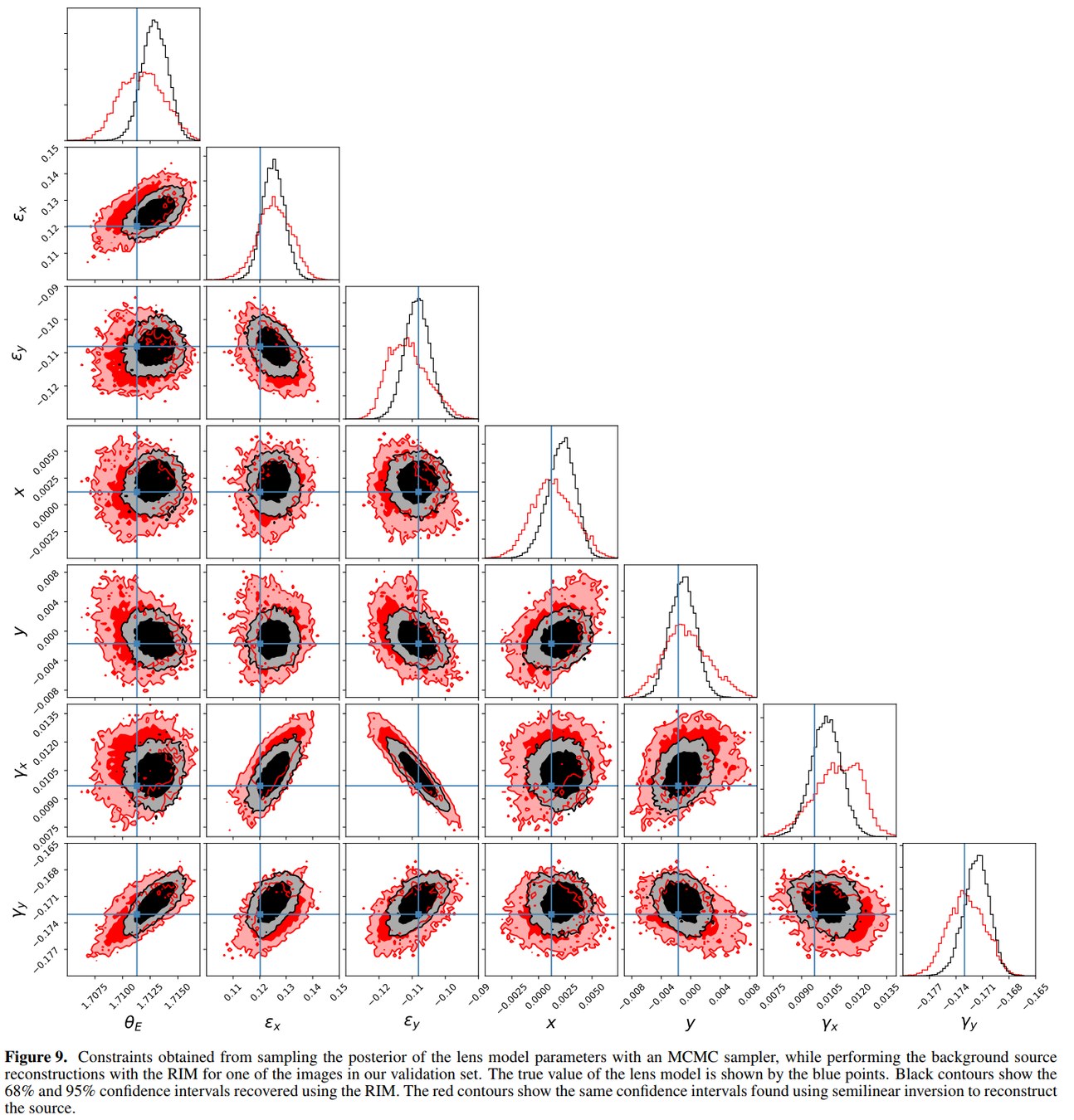
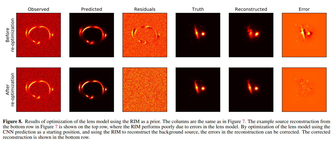
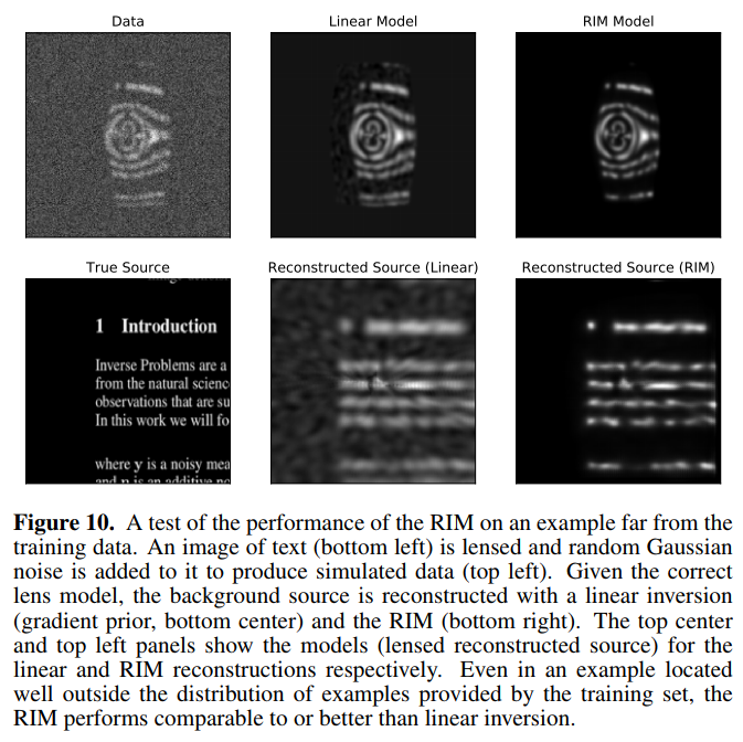
Data-Driven Reconstruction of Gravitationally Lensed Galaxies using Recurrent Inference Machines
Morningstar et al. 2019
Inverting Strong Gravitational Lensing

Recurrent Inferrence Machines
By eiffl
Recurrent Inferrence Machines
Session on RIMs for the Berkeley Statistics and Machine Learning Forum


