


Steven De Keninck PRO
Mathematical Experimentalist
Geometric Algebra
The Prequel.
Steven De Keninck & Martin Roelfs
What is Geometric Algebra ?
An alternative to vector/matrix algebra ideal for (amongst many other things) geometry.
An algebra on a graded linear (vector) space, with an invertible product that operates on multivectors.
\(\oplus\)
\(\oplus\)
\(\circlearrowleft\)
\(\oplus\)
\(\oplus\)
\(\mathbb R\)
...
PSS
scalars
vectors
bivectors
pseudo scalar
What is Geometric Algebra ?
We will first tackle the Algebra.
الكتاب المختصر في حساب الجبر والمقابلة
al-Kitāb al-Mukhtaṣar fī Ḥisāb al-Jabr wal-Muqābalah
The Compendious Book on Calculation by Completion and Balancing
1. New Numbers: why do we need them?
1. New Numbers: why do we need them?
\(x^2 + 10x = 39\)
\(= 39\)
\(+ 25=64\)
\((x+5)^2 = 64\)
\(\Leftrightarrow x = 3\)
\(x\)
\(x\)
\(x^2\)
\(x\)
\(5\)
\(5x\)
\(x\)
\(5\)
\(5x\)
\(5\)
\(5\)
\(25\)
\( \begin{cases} \\ \\ \\ \\ \\ \\ \\ \\ \\ \\ \end{cases}\)
\(x+5\)
1. New Numbers: why do we need them?
\(ax^2 = bx\)
\(ax^2 = c\)
\(bx = c\)
\(ax^2 + bx = c\)
\(ax^2+c = bx\)
\(bx + c = ax^2\)
Why six equations ?????
No negative numbers, no zero !!
1. New Numbers: why do we need them?
Why six equations ?????
No negative numbers, no zero !!
\(x + 1 = 1\)
\(x + 1 = 0\)
zero!
negative numbers!
With 0 and negative numbers, we reduce the amount of equations from 6 to 1 !!!
\(\oplus\)
\(\oplus\)
\(\circlearrowleft\)
\(\oplus\)
\(\oplus\)
\(\mathbb R\)
...
PSS
scalars
vectors
bivectors
pseudo scalar
Transform point/line/plane/direction \(b\) with rotor \(a\)
\(ab\tilde a\)
Project any point/line/plane \(a\) on any point/line/plane \(b\)
\(\frac {a\cdot b} {b}\)
Compare this to the classic vector/matrix approach ...
// just a matrix multiply
transform_point( M,  )
// similar to point .. diff. M
transform_direction( M,  )
// should be 6x6 matrix
transform_line( M,  )
// similar to direction .. diff. M
transform_plane( M,  )
// none of these are similar..
project_point_line()
project_point_plane()
project_line_point()
project_line_plane()
project_plane_point()
project_plane_line()Lets do the same with another simple equation..
e
e
e
\(\mathbf e^2 = -1\)
\(\mathbf e^2 = +1\)
\(\mathbf e^2 = 0\)
\(\mathbb R_{\color{green}p\color{white},\color{red}q\color{white},\color{cyan}r\color{white}}\)
A Geometric Algebra is defined by this p,q,r signature specifying the metric of the n generators.
2. New Numbers: what are they?
\(\oplus\)
\(\oplus\)
\(\circlearrowleft\)
\(\oplus\)
\(\oplus\)
\(\mathbb R\)
...
PSS
scalars
vectors
bivectors
pseudo scalar
Transform point/line/plane/direction \(b\) with rotor \(a\)
\(ab\tilde a\)
Project any point/line/plane \(a\) on any point/line/plane \(b\)
\(\frac {a\cdot b} {b}\)
\(\mathbb R_{\color{green}p\color{white},\color{red}q\color{white},\color{cyan}r\color{white}}\)
A Geometric Algebra is defined by this p,q,r signature specifying the metric of the n generators.
\(\mathbf e_1, \mathbf e_2, \mathbf e_3 \), all square to \(+1\)
\(\mathbf e_1\) squares to \(+1\), \(\mathbf e_2, \mathbf e_3, \mathbf e_4\), all square to \(-1\)
\(\mathbf e_0\) squares to \(0\), \(\mathbf e_1, \mathbf e_2 ,\mathbf e_3\), all square to \(+1\)
We will use these generators to model vectors, points, circles, lines, planes, translations, boosts, rotations, screws, spheres, ...
\( \mathbf e_i \notin \mathbb R \qquad {\mathbf e_i}^2 \in \{0,1,-1\} \)
2. New Numbers: what are they?
3. New Numbers: how do I use them?
\( \mathbf e_i \notin \mathbb R \qquad {\mathbf e_i}^2 \in \{0,1,-1\} \)
\(x^2 \in \mathbb R\)
\((\alpha \mathbf e_1 + \beta \mathbf e_2)^2 \in \mathbb R\)
\(\alpha^2 \mathbf {e_1}^2 + \alpha\beta\color{lightgreen}\mathbf e_1\mathbf e_2\color{white} + \alpha\beta\color{lightgreen}\mathbf e_2\mathbf e_1 \color{white} + \beta^2 {\mathbf e_2}^2 \in \mathbb R\)
\( \color{lightgreen} \mathbf e_1\mathbf e_2 + \mathbf e_2\mathbf e_1 \color{white} = 0\)
\( \mathbf e_1\mathbf e_2 = - \mathbf e_2\mathbf e_1 \color{white} \)
\(\mathbf e_1\)
\(\mathbf e_2\)
\(x = \alpha \mathbf e_1 + \beta \mathbf e_2\)
\( \mathbf e_i \notin \mathbb R \qquad {\mathbf e_i}^2 \in \{0,1,-1\} \)
\( \mathbf e_1\mathbf e_2 = - \mathbf e_2\mathbf e_1 \)
3. New Numbers: how do I use them?
What is this new \(\mathbf e_1 \mathbf e_2 = \mathbf e_{12}\) element?
\(\alpha\mathbf e_1 + \beta\mathbf e_2\)
\(\alpha\mathbf e_{12}\)
\(\alpha\mathbf e_{12}\)
\(\alpha\mathbf e_{123}\)
\( \mathbf e_i \notin \mathbb R \qquad {\mathbf e_i}^2 \in \{0,1,-1\} \)
\( \mathbf e_1\mathbf e_2 = - \mathbf e_2\mathbf e_1 \)
3. New Numbers: how do I use them?
\((\mathbf e_1 - \mathbf e_2)\mathbf e_1 = \)
\({\mathbf e_{12}}^2 = \)
\(\mathbf e_{123}\mathbf e_1 =\)
\(\frac 1 2 (\mathbf e_1 + \mathbf e_2) (\mathbf e_2 - \mathbf e_1) = \)
some exercises, with positive basis vectors.
\(\bf \frac 1 2 (e_{12} - 1 + 1 -e_{21} ) = e_{12}\)
\(\curvearrowleft\)
\(\bf e_{1231} = -e_{1213} = e_{1123} = e_{23}\)
\(\curvearrowleft\)
\(\curvearrowleft\)
\(\bf e_1e_1 - e_2e_1 = 1 + e_{12}\)
\(\curvearrowleft\)
\(\curvearrowleft\)
\(\bf e_{12} e_{12} = e_{1212} = - e_{1221} = -1\)
\( \mathbf e_i \notin \mathbb R \qquad {\mathbf e_i}^2 \in \{0,1,-1\} \)
\( \mathbf e_1\mathbf e_2 = - \mathbf e_2\mathbf e_1 \)
3. New Numbers: how do I use them?
The geometric product of two 3 dimensional vectors
\(v_1v_2 = (\color{lightblue}x_1\color{white}\color{lightgreen}x_2\color{white}+\color{lightblue}y_1\color{white}\color{lightgreen}y_2\color{white}+\color{lightblue}z_1\color{white}\color{lightgreen}z_2\color{white}) + (\color{lightblue}x_1\color{white}\color{lightgreen}y_2\color{white}-\color{lightblue}y_1\color{white}\color{lightgreen}x_2\color{white})\mathbf e_{12} + (-\color{lightblue}x_1\color{white}\color{lightgreen}z_2\color{white}+\color{lightblue}z_1\color{white}\color{lightgreen}x_2\color{white})\mathbf e_{31} + (\color{lightblue}y_1\color{white}\color{lightgreen}z_2\color{white}-\color{lightblue}z_1\color{white}\color{lightgreen}y_2\color{white})\mathbf e_{23}\)
\(\vec v_1 = \begin{bmatrix}\color{lightblue}x_1 \\ \color{lightblue} y_1 \\ \color{lightblue} z_1 \color{white} \end{bmatrix} \quad \vec v_2 = \begin{bmatrix}\color{lightgreen}x_2 \\ \color{lightgreen} y_2 \\ \color{lightgreen} z_2 \color{white} \end{bmatrix}\)
\( \underbrace{\qquad \qquad\qquad\qquad\qquad\qquad\qquad\qquad\qquad\qquad\qquad}\)
\( \cong \vec v_1 \times \vec v_2 \)
Cross Product !
\( \underbrace{\qquad \qquad\qquad\qquad}\)
\( \cong \vec v_1 \cdot \vec v_2 \)
Dot Product !
\(v_1 = (\color{lightblue}x_1\color{white}\mathbf e_{1} + \color{lightblue}y_1\color{white}\mathbf e_{2} + \color{lightblue}z_1\color{white}\mathbf e_{3} )\)
\(v_2 = ( \color{lightgreen}x_2\color{white}\mathbf e_{1} + \color{lightgreen}y_2\color{white}\mathbf e_{2} + \color{lightgreen}z_2\color{white}\mathbf e_{3})\)
\( \mathbf e_i \notin \mathbb R \qquad {\mathbf e_i}^2 \in \{0,1,-1\} \)
\( \mathbf e_1\mathbf e_2 = - \mathbf e_2\mathbf e_1 \)
3. New Numbers: how do I use them?
The geometric product of two 3 dimensional vectors
\(v_1v_2 = (\color{lightblue}x_1\color{white}\color{lightgreen}x_2\color{white}+\color{lightblue}y_1\color{white}\color{lightgreen}y_2\color{white}+\color{lightblue}z_1\color{white}\color{lightgreen}z_2\color{white}) + (\color{lightblue}x_1\color{white}\color{lightgreen}y_2\color{white}-\color{lightblue}y_1\color{white}\color{lightgreen}x_2\color{white})\mathbf e_{12} + (-\color{lightblue}x_1\color{white}\color{lightgreen}z_2\color{white}+\color{lightblue}z_1\color{white}\color{lightgreen}x_2\color{white})\mathbf e_{31} + (\color{lightblue}y_1\color{white}\color{lightgreen}z_2\color{white}-\color{lightblue}z_1\color{white}\color{lightgreen}y_2\color{white})\mathbf e_{23}\)
\( \underbrace{\qquad \qquad\qquad\qquad\qquad\qquad\qquad\qquad\qquad\qquad\qquad}\)
\( \cong \vec v_1 \times \vec v_2 \)
Cross Product !
\( \underbrace{\qquad \qquad\qquad\qquad}\)
\( \cong \vec v_1 \cdot \vec v_2 \)
Dot Product !
only scalar. 'Grade 0'.
\(v_1 \cdot v_2 = \langle v_1v_2 \rangle_0\)
only bivector. 'Grade 2'.
\(v_1 \wedge v_2 = \langle v_1v_2 \rangle_2\)
Note : One scalar and three imaginary parts. The geometric product of two vectors in \(\mathbb R_3\) is a quaternion!
\( \mathbf e_i \notin \mathbb R \qquad {\mathbf e_i}^2 \in \{0,1,-1\} \)
\( \mathbf e_1\mathbf e_2 = - \mathbf e_2\mathbf e_1 \)
3. New Numbers: how do I use them?
The geometric product of two 3 dimensional vectors
\(v_1v_2 = (\color{lightblue}x_1\color{white}\color{lightgreen}x_2\color{white}+\color{lightblue}y_1\color{white}\color{lightgreen}y_2\color{white}+\color{lightblue}z_1\color{white}\color{lightgreen}z_2\color{white}) + (\color{lightblue}x_1\color{white}\color{lightgreen}y_2\color{white}-\color{lightblue}y_1\color{white}\color{lightgreen}x_2\color{white})\mathbf e_{12} + (-\color{lightblue}x_1\color{white}\color{lightgreen}z_2\color{white}+\color{lightblue}z_1\color{white}\color{lightgreen}x_2\color{white})\mathbf e_{31} + (\color{lightblue}y_1\color{white}\color{lightgreen}z_2\color{white}-\color{lightblue}z_1\color{white}\color{lightgreen}y_2\color{white})\mathbf e_{23}\)
only scalar. 'Grade 0'.
\(v_1 \cdot v_2 = \langle v_1v_2 \rangle_0\)
only bivector. 'Grade 2'.
\(v_1 \wedge v_2 = \langle v_1v_2 \rangle_2\)
\(v_1v_2 = v_1 \cdot v_2 + v_1 \wedge v_2 \)
*famous, but be careful! only if \(v_1\) or \(v_2\) is vector!
\( \mathbf e_i \notin \mathbb R \qquad {\mathbf e_i}^2 \in \{0,1,-1\} \)
\( \mathbf e_1\mathbf e_2 = - \mathbf e_2\mathbf e_1 \)
3. New Numbers: how do I use them?
\(v_1v_2 = v_1 \cdot v_2 + v_1 \wedge v_2 \)
In general, the geometric product between a grade \(s\) multivector \(\bf a\) and a grade \(t\) multivector \(\bf b\) has grades from \(|s-t|\) to \(s+t\) in steps of 2.
The highest and lowest grade parts are often useful and are called the wedge and dot products respectively.
\( \langle a \rangle_s \cdot \langle b \rangle_t = \langle ab \rangle_{|s-t|}\)
\( \langle a \rangle_s \wedge \langle b \rangle_t = \langle ab \rangle_{s+t}\)
\( \mathbf e_i \notin \mathbb R \qquad {\mathbf e_i}^2 \in \{0,1,-1\} \)
\( \mathbf e_1\mathbf e_2 = - \mathbf e_2\mathbf e_1 \)
3. New Numbers: how do I use them?
There are even more products from other branches of mathematics and physics
that map to some combination of or grade selection of the geometric product!
\( \langle a \rangle_s \cdot \langle b \rangle_t = \langle ab \rangle_{|s-t|}\)
\( \langle a \rangle_s \wedge \langle b \rangle_t = \langle ab \rangle_{s+t}\)
\(( a \vee b)^* = a^* \wedge b^*\)
\( a \times b = \frac 1 2 (ab - ba)\)
The Geometric Product
The Wedge Product
The Dot Product
The Vee Product
The Commutator Product
\(\oplus\)
\(\oplus\)
\(\circlearrowleft\)
\(\oplus\)
\(\oplus\)
\(\mathbb R\)
...
PSS
scalars
vectors
bivectors
pseudo scalar
4. Cayley Tables !
\( \mathbf e_i \notin \mathbb R \qquad {\mathbf e_i}^2 \in \{0,1,-1\} \)
\( \mathbf e_1\mathbf e_2 = - \mathbf e_2\mathbf e_1 \)
\(\oplus\)
\(\oplus\)
\(\circlearrowleft\)
\(\oplus\)
\(\oplus\)
\(\mathbb R\)
...
PSS
scalars
vectors
bivectors
pseudo scalar
4. SpaceTime Algebra!
\( \mathbf e_i \notin \mathbb R \qquad {\mathbf e_i}^2 \in \{0,1,-1\} \)
\( \mathbf e_1\mathbf e_2 = - \mathbf e_2\mathbf e_1 \)
The geometric numbers allow us to mix and match to create a number of interesting geometric algebras
\(\mathbb R_{1,3} \)
Spacetime Algebra or STA
physicist favorite!
\(\begin{aligned} \gamma_0 &= \begin{bmatrix} 1 & 0 & 0 & 0 \\ 0 & 1 & 0 & 0 \\ 0 & 0 & -1 & 0 \\ 0 & 0 & 0 & -1 \end{bmatrix} \ \gamma_1 &= \begin{bmatrix} 0 & 0 & 0 & 1 \\ 0 & 0 & 1 & 0 \\ 0 & -1 & 0 & 0 \\ -1 & 0 & 0 & 0 \end{bmatrix} \ \\ \gamma_2 &= \begin{bmatrix} 0 & 0 & 0 & -i \\ 0 & 0 & i & 0 \\ 0 & i & 0 & 0 \\ -i & 0 & 0 & 0 \end{bmatrix} \ \gamma_3 &= \begin{bmatrix} 0 & 0 & 1 & 0 \\ 0 & 0 & 0 & -1 \\ -1 & 0 & 0 & 0 \\ 0 & 1 & 0 & 0 \end{bmatrix} \end{aligned}\)
\(\sigma_1 = \begin{bmatrix} 0 & 1 \\ 1 & 0 \end{bmatrix} \ \sigma_2 = \begin{bmatrix} 0 & -i \\ i & 0 \end{bmatrix} \ \sigma_3 = \begin{bmatrix} 1 & 0 \\ 0 & -1 \end{bmatrix}\)
\(\gamma_0 = \mathbf e_0\,\, \gamma_1 = \mathbf e_1\,\, \gamma_2 = \mathbf e_2\,\, \gamma_3 = \mathbf e_3 \)
\(\sigma_i = \gamma_i \gamma_0 \implies \newline \sigma_1 = \mathbf e_{10},\,\,\,\sigma_2 = \mathbf e_{20},\,\,\,\sigma_3 = \mathbf e_{30} \)
\(I = \gamma_0 \gamma_1 \gamma_2 \gamma_3 = \sigma_1 \sigma_2 \sigma_3\)
\(\oplus\)
\(\oplus\)
\(\circlearrowleft\)
\(\oplus\)
\(\oplus\)
\(\mathbb R\)
...
PSS
scalars
vectors
bivectors
pseudo scalar
\( \mathbf e_i \notin \mathbb R \qquad {\mathbf e_i}^2 \in \{0,1,-1\} \)
\( \mathbf e_1\mathbf e_2 = - \mathbf e_2\mathbf e_1 \)
The geometric numbers allow us to mix and match to create a number of interesting geometric algebras
\(\mathbb R_{1,3} \)
Spacetime Algebra or STA
physicist favorite!
\(\begin{aligned} \gamma_0 &= \begin{bmatrix} 1 & 0 & 0 & 0 \\ 0 & 1 & 0 & 0 \\ 0 & 0 & -1 & 0 \\ 0 & 0 & 0 & -1 \end{bmatrix} \to \mathbf{e}_1, \quad \gamma_1 &= \begin{bmatrix} 0 & 0 & 0 & 1 \\ 0 & 0 & 1 & 0 \\ 0 & -1 & 0 & 0 \\ -1 & 0 & 0 & 0 \end{bmatrix} \to \mathbf{e}_2 \\ \gamma_2 &= \begin{bmatrix} 0 & 0 & 0 & -i \\ 0 & 0 & i & 0 \\ 0 & i & 0 & 0 \\ -i & 0 & 0 & 0 \end{bmatrix} \to \mathbf{e}_3, \quad \gamma_3 &= \begin{bmatrix} 0 & 0 & 1 & 0 \\ 0 & 0 & 0 & -1 \\ -1 & 0 & 0 & 0 \\ 0 & 1 & 0 & 0 \end{bmatrix} \to \mathbf{e}_4\end{aligned}\)
\(\sigma_1 = \begin{bmatrix} 0 & 1 \\ 1 & 0 \end{bmatrix}, \quad \sigma_2 = \begin{bmatrix} 0 & -i \\ i & 0 \end{bmatrix}, \quad \sigma_3 = \begin{bmatrix} 1 & 0 \\ 0 & -1 \end{bmatrix}\)
\(\sigma_i = \gamma_i \gamma_0 \)
\(\mathbb R_{3} \cong \mathbb R_{1,3}^+ \)
4. SpaceTime Algebra!
\(\oplus\)
\(\oplus\)
\(\circlearrowleft\)
\(\oplus\)
\(\oplus\)
\(\mathbb R\)
...
PSS
scalars
vectors
bivectors
pseudo scalar
\( \mathbf e_i \notin \mathbb R \qquad {\mathbf e_i}^2 \in \{0,1,-1\} \)
\( \mathbf e_1\mathbf e_2 = - \mathbf e_2\mathbf e_1 \)
The spacetime split is a mapping between 3D space and STA using \(\sigma_i = \gamma_i \gamma_0 \).
4. SpaceTime Algebra!
4. SpaceTime Algebra!
time
space
\(\oplus\)
\(\oplus\)
\(\circlearrowleft\)
\(\oplus\)
\(\oplus\)
\(\mathbb R\)
...
PSS
scalars
vectors
bivectors
pseudo scalar
\( \mathbf e_i \notin \mathbb R \qquad {\mathbf e_i}^2 \in \{0,1,-1\} \)
\( \mathbf e_1\mathbf e_2 = - \mathbf e_2\mathbf e_1 \)
The spacetime split is a mapping between 3D space and STA using \(\sigma_i = \gamma_i \gamma_0 \).
The definitive example of the power of the spacetimeis the singular Maxwell equation:
$$ \partial F = J \quad \implies \quad \partial \cdot F = J \quad \partial \wedge F = 0 $$
where \(\partial = \gamma^\mu \partial_\mu\) is the gradient operator, \(J = \gamma^\mu J_\mu\) is the source term, and \( F = \mathbf{E} + I \mathbf{B} \) is the field strength bivector. To prove that this indeed reproduces the familiar Maxwell equations, we use the spacetime split:
$$ \begin{aligned} J \gamma_0 &= J \cdot \gamma_0 + J \wedge \gamma_0 = \rho + \mathbf{J} \\ \partial \gamma_0 &= \partial \cdot \gamma_0 + \partial \wedge \gamma_0 = \partial_t + \nabla \end{aligned} $$
Most compact form of the Maxwell equations!
\(\partial \cdot F = J \leftrightarrow \partial_\alpha F^{\alpha \beta} = J^\beta\)
\(\partial \wedge F = 0 \leftrightarrow \partial_\alpha (\tfrac{1}{2} \epsilon^{\alpha\beta\gamma\delta}F_{\gamma\delta}) = 0\)
4. SpaceTime Algebra!
4. SpaceTime Algebra!
Projective or 'Plane-based' Geometric Algebra uses an extra basis vector to model elements at infinity. This enables a unification of rotations and translations, exception-free incidence, covariant transformations and more!
4. PGA - Projective Geometric Algebra
\(\mathbb R_{3,0,1}\)
\(\mathbb R_{4}\)
\(\mathbb R_{3,1}\)
FLAT
SPHERICAL
HYPERBOLIC
Felix Klein - Erlangen Program
\( ab \)
compose any a,b
\( a\wedge b \)
intersect any a,b
\( a\vee b \)
join any a,b
\( (a\cdot b)b^{-1} \)
project any a onto/into b
for any point/line/plane a,b
Projective or 'Plane-based' Geometric Algebra uses an extra basis vector to model elements at infinity. This enables a unification of rotations and translations, exception-free incidence, covariant transformations and more!
4. PGA - Projective Geometric Algebra
\(\mathbb R_{n,0,1}\)
\(\mathbb R_{n+1}\)
\(\mathbb R_{n,1}\)
FLAT
SPHERICAL
HYPERBOLIC
\( ab \)
compose any a,b
\( a\wedge b \)
intersect any a,b
\( a\vee b \)
join any a,b
\( (a\cdot b)b^{-1} \)
project any a onto/into b
for any point/line/plane a,b
A very natural language to describe the geometry of points, lines and planes.
(can be bent into the conformal group and the geometry of spheres, circles and point-pairs)
\(\oplus\)
\(\oplus\)
\(\circlearrowleft\)
\(\oplus\)
\(\oplus\)
\(\mathbb R\)
...
PSS
scalars
vectors
bivectors
pseudo scalar
Prequel : Recap!
\( \mathbf e_i \notin \mathbb R \qquad {\mathbf e_i}^2 \in \{0,1,-1\} \)
\( \mathbf e_1\mathbf e_2 = - \mathbf e_2\mathbf e_1 \)
\( \langle a \rangle_s \cdot \langle b \rangle_t = \langle ab \rangle_{|s-t|}\)
\( \langle a \rangle_s \wedge \langle b \rangle_t = \langle ab \rangle_{s+t}\)
\(( a \vee b)^* = a^* \wedge b^*\)
\( a \times b = \frac 1 2 (ab - ba)\)
Geometric Product
Wedge
Dot
Vee
Commutator
\(\oplus\)
\(\oplus\)
\(\circlearrowleft\)
\(\oplus\)
\(\oplus\)
\(\mathbb R\)
...
PSS
scalars
vectors
bivectors
pseudo scalar
Prequel : Recap!
Congratulations! You are now ready for geometry.
\(\oplus\)
\(\oplus\)
\(\circlearrowleft\)
\(\oplus\)
\(\oplus\)
\(\mathbb R\)
...
PSS
scalars
vectors
bivectors
pseudo scalar
Transform point/line/plane/direction \(b\) with rotor \(a\)
\(ab\tilde a\)
Project any point/line/plane \(a\) on any point/line/plane \(b\)
\(\frac {a\cdot b} {b}\)
1. New Numbers: what are they?
The Key? Geometric Numbers.
e
e
e
\(\mathbb R_{\color{green}p\color{white},\color{red}q\color{white},\color{cyan}r\color{white}}\)
The set we work with is generated by the real numbers, p positive, q negative and r null basis elements, conveniently called \(\mathbf e_i\)
\(\mathbf e^2 = -1\)
\(\mathbf e^2 = +1\)
\(\mathbf e^2 = 0\)
In PGA these new numbers e represent reflections
Euclidean geometry is the geometry of the Euclidean group Felix Klein
All transformations and elements in PGA are build by composing reflections.
Plane-based Geometric Algebra
\(\mathbf e^2 = -1\)
\(\mathbf e^2 = +1\)
\(\mathbf e^2 = 0\)
In PGA these new numbers e represent reflections
Euclidean geometry is the geometry of the Euclidean group Felix Klein
All transformations and elements in PGA are build by composing reflections.
Parallel Bireflection
Identical Bireflection
Intersecting Bireflection
Translation
Identity
Rotation
Bireflections have a gauge degree of freedom.
We study the composition of two reflections called a bireflection
Plane-based Geometric Algebra
When we combine \(3\) reflections, we get glide-reflections, and can always gauge it into a translation+reflection.
We can now gauge to make all mirrors orthogonal
So each trireflection is a translation and reflection along/in the same line.
Plane-based Geometric Algebra
When we combine \(k\) reflections, we get \(k-1\) of these geometric gauges.
We can now gauge to make the grey mirrors overlap.
Identical mirrors vanish.
This happens automatically during composition.
Plane-based Geometric Algebra
When we combine \(k\) reflections, we get \(k-1\) of these geometric gauges.
We can now gauge to make the grey mirrors overlap.
Identical mirrors vanish.
This happens automatically during composition.
| 0 | identity |
| 1 | reflection |
| 2 | translation/rotation |
| 3 | glide reflection |
| 4 | ⟶2 |
Plane-based Geometric Algebra
When we combine \(k\) reflections, we get \(k-1\) of these geometric gauges.
| 0 | identity |
| 1 | reflection |
| 2 | translation |
| 3 | ⟶1 |
Visualizing 1D PGA
in 1D the situation is simple. We only have point reflections · and translations · ·
We want to have the same meaning for these elements in arbitrary dimensions, so we can use 1D techniques for any 1D subspace in nD
All elements in 1D PGA are visualized with at most 2 points.
•
••
Plane-based Geometric Algebra
Visualizing 2D PGA
| 0 | identity |
| 1 | reflection |
| 2 | translation/rotation |
| 3 | glide reflection |
| 4 | ⟶2 |
lines
points
translations
rotations
/
// X
// /
All elements of 2D PGA can be visualized as lines
1D
Plane-based Geometric Algebra
Visualizing 3D PGA
planes \
lines +
points ⚹
translations \\
rotations X
| 0 | identity |
| 1 | reflection |
| 2 | translation/rotation |
| 3 | glide/roto reflection |
| 4 | screw motion |
| 5 | ⟶3 |
\
\\ X
\X
\\X
1D
2D
Plane-based Geometric Algebra
By design, ideas from n-d are transplanted to work in (n+1)-d.
The structure of n-d PGA is exactly correct to get dimension-independent operators!
1D
2D
3D
Plane-based Geometric Algebra
The structure of n-d PGA is exactly correct to get dimension-independent operators!
There is one plane for each plane reflection, one line for each line reflection, one point for each point reflection.
1D
2D
3D
Plane-based Geometric Algebra
The elements and transformations of nD PGA are all k-reflections!
points = point-reflections
lines = line-reflections
planes = plane-reflections
These elements all are their own inverse .. they are all geometric numbers (\(a^2 = \pm1\)).
\( aa \tilde a = \pm a \)
all these elements are invariant under their associated transormations.
3D
Plane-based Geometric Algebra
3D
The elements and transformations of nD PGA are all k-reflections!
points = point-reflections
lines = line-reflections
planes = plane-reflections
These elements all are their own inverse .. they are all geometric numbers (\(a^2 = \pm1\)).
\( aa \tilde a = \pm a \)
all these elements are invariant under their associated transormations.
This makes it easy to find transformations that relate elements, using nothing but composition.
PP = translation
ll = rotation/translation/screw
pp = rotation/translation
But they produce twice the transformation we need - so we need a way to take square roots (\(\sqrt{x}=x^{\frac 1 2}\)), and with general powers we can generate general rotations/translations
\( \sqrt{ab} = \overline{1+ab} \)
\( (ab)^{\alpha} = e^{\alpha \log{ab}} \)
Plane-based Geometric Algebra
Lets look at a classic - gluLookAt
void GLAPIENTRY
gluLookAt(GLdouble eyex, GLdouble eyey, GLdouble eyez, GLdouble centerx,
      GLdouble centery, GLdouble centerz, GLdouble upx, GLdouble upy,
      GLdouble upz)
{
    float forward[3], side[3], up[3];
    GLfloat m[4][4];

    forward[0] = centerx - eyex;
    forward[1] = centery - eyey;
    forward[2] = centerz - eyez;

    up[0] = upx;
    up[1] = upy;
    up[2] = upz;

    normalize(forward);

    /* Side = forward x up */
    cross(forward, up, side);
    normalize(side);

    /* Recompute up as: up = side x forward */
    cross(side, forward, up);

    __gluMakeIdentityf(&m[0][0]);
    m[0][0] = side[0];
    m[1][0] = side[1];
    m[2][0] = side[2];

    m[0][1] = up[0];
    m[1][1] = up[1];
    m[2][1] = up[2];

    m[0][2] = -forward[0];
    m[1][2] = -forward[1];
    m[2][2] = -forward[2];

    glMultMatrixf(&m[0][0]);
    glTranslated(-eyex, -eyey, -eyez);
}
Inputs
Output
\(r_1\)
\(r_2\)
\(r_3\)
\( M = 1, P = 1^* \)
\(P = \overline{P \vee p_i}\)
\( M = \sqrt{PMr_i\tilde M} M \)
\(p_1\)
\(p_2\)
\(p_3\)
Plane-based Geometric Algebra
Lets look at a classic - gluLookAt
// input  : p = array of euclidean/infinite points
// output : motor that aligns the reference frame to p

function align(p) {
  var M=1, P=!1;
  for (var i=0; i<p.length; ++i) {
    P = (P & p[i]).Normalized;
    M = sqrt(P * (M >>> r[i])) * M;
  }
  return M
}
\( M = 1, P = 1^* \)
\(P = \overline{P \vee p_i}\)
\( M = \sqrt{PMr_i\tilde M} M \)
Plane-based Geometric Algebra
Thank you.
https://bivector.net
Plane-based Geometric Algebra
PGA
A
B
C
Motivation + intuition
Steven
Algebraic foundation
Leo
Applications: IK + RBD
Steven
| A | B | A | B | C | C |
|---|
Plane-based Geometric Algebra
Episode 1 : The Reflection Menace
Episode 2 : Attack of the Mirrors
Episode 3 : Revenge of Infinity
Episode 4 : The Forque Awakens
Episode 5 : A New Hope I
Episode 6 : A New Hope II
Plane-based Geometric Algebra
What is Geometric Algebra ?
An alternative to vector/matrix algebra ideal for (computer) geometry.
An algebra on a graded linear (vector) space, with an invertible product that operates on multivectors.
\(\oplus\)
\(\oplus\)
\(\circlearrowleft\)
\(\oplus\)
\(\oplus\)
\(\mathbb R\)
...
PSS
scalars
vectors
bivectors
pseudo scalar
Transform any point/line/plane/... \(b\) with any rotor \(a\)
\(ab\tilde a\)
Project any point/line/plane \(a\) on any point/line/plane \(b\)
\(\frac {a\cdot b} {b}\)
Plane-based Geometric Algebra
What is Geometric Algebra ?
An alternative to vector/matrix algebra ideal for (computer) geometry.
\(\oplus\)
\(\oplus\)
\(\circlearrowleft\)
\(\oplus\)
\(\oplus\)
\(\mathbb R\)
...
PSS
scalars
vectors
bivectors
pseudo scalar
Transform point/line/plane/direction \(b\) with rotor \(a\)
\(ab\tilde a\)
Project any point/line/plane \(a\) on any point/line/plane \(b\)
\(\frac {a\cdot b} {b}\)
Compare this to the classic vector/matrix approach ...
// just a matrix multiply
transform_point( M,  )
// similar to point .. diff. M
transform_direction( M,  )
// should be 6x6 matrix
transform_line( M,  )
// similar to direction .. diff. M
transform_plane( M,  )
// none of these are similar..
project_point_line()
project_point_plane()
project_line_point()
project_line_plane()
project_plane_point()
project_plane_line()Plane-based Geometric Algebra
Coordinate free and Dimension agnostic.
We do not commonly expect to be able to download e.g. a 2D physics engine and change the number of dimensions to 3.
Constructions and products that are only valid in 3D are commonly used in the description of geometry and physics. (e.g. the cross product)
Can we do better?
on a need to know basis
Plane-based Geometric Algebra
What is Geometric Algebra ?
An alternative to vector/matrix algebra ideal for (computer) geometry.
\(\oplus\)
\(\oplus\)
\(\circlearrowleft\)
\(\oplus\)
\(\oplus\)
\(\mathbb R\)
...
PSS
scalars
vectors
bivectors
pseudo scalar
this is not a vector.
ceci n'est pas un vecteur
this is a vector.
how many dimensions ?
does it have an orientation ?
\( x^2 = \lVert x \rVert^2 \)
only its length is well defined.
Coordinate free and Dimension agnostic.
Plane-based Geometric Algebra
What is Geometric Algebra ?
An alternative to vector/matrix algebra ideal for (computer) geometry.
\(\oplus\)
\(\oplus\)
\(\circlearrowleft\)
\(\oplus\)
\(\oplus\)
\(\mathbb R\)
...
PSS
scalars
vectors
bivectors
pseudo scalar
\( x^2 = \lVert x \rVert^2 \)
When a second non colinear vector is added
There is more to being dimension agnostic, but not having an origin and coordinate axes is a good starting point. Logic with points, lines, planes should work independent of the dimensionality of the space!
Coordinate free and Dimension agnostic.
Plane-based Geometric Algebra
What is Geometric Algebra ?
An alternative to vector/matrix algebra ideal for (computer) geometry.
\(\oplus\)
\(\oplus\)
\(\circlearrowleft\)
\(\oplus\)
\(\oplus\)
\(\mathbb R\)
...
PSS
scalars
vectors
bivectors
pseudo scalar
There is more to being dimension agnostic, but not having an origin and coordinate axes is a good starting point. Logic with points, lines, planes should work independent of the dimensionality of the space!
Coordinate free and Dimension agnostic.
\(a\)
\(b\)
Expressions that involve \(a,b,c\) should not depend on the # of coefficients used to describe them :
\(c\)
The First Postulate
Steven De Keninck
The First Postulate
In this talk:
The First Postulate
\(\mathbb R_{3,0,1}\)
\(3\) basis vectors \(\mathbf e_1, \mathbf e_2, \mathbf e_3\)
\(1\) null basis vector \(\mathbf e_0\)
\( \mathbf e_i \notin \mathbb R \qquad {\mathbf e_i}^2 \in \{1,-1,0\} \)
\( \mathbf e_1\mathbf e_2 = - \mathbf e_2\mathbf e_1 \)
\(\mathbf e_0, \mathbf e_1, \mathbf e_2, \mathbf e_3\)
\(\mathbf e_{01},\mathbf e_{02},\mathbf e_{03}, \mathbf e_{12}, \mathbf e_{31}, \mathbf e_{23}\)
\(\mathbf e_{021},\mathbf e_{013},\mathbf e_{032}, \mathbf e_{123}\)
\( \mathbf e_{0123}\)
\( \mathbf 1\)
→ scalar
→ vector
→ bivector
→ trivector
→ pseudo-scalar
vector = linear comb of generators
\(\begin{bmatrix}x \\ y \\ z \\ w \end{bmatrix} \rightarrow x\mathbf e_1 + y\mathbf e_2 + z\mathbf e_3 + w\mathbf e_0\)
bivectors \(e_{ij}\), trivectors \(e_{ijk}\), ...
multivector = sum of k-vectors
\(\vec a \vec b = \vec a \cdot \vec b + \vec a \wedge \vec b\)
\(\langle a\rangle_k\) selects grade \(k\) of \(a\)
skipping many aspects here: reverses, inverses, dualization, exponentials and logarithms, natural inclusion of (dual) quaternions, Lie algebras, etc ...
\( \langle a \rangle_s \langle b \rangle_t = \langle ab \rangle_{|s-t|}+ ... + \langle ab \rangle_{s+t}\)
The Geometric Product
\( \langle a \rangle_s \wedge \langle b \rangle_t = \langle ab \rangle_{s+t}\)
The Wedge Product
\( \langle a \rangle_s \cdot \langle b \rangle_t = \langle ab \rangle_{|s-t|}\)
The Dot Product
\(( a \vee b)^* = a^* \wedge b^*\)
The Vee Product
\(-1^{st} \langle a \rangle_s \langle b \rangle_t \widetilde{\langle a \rangle_s}\)
The Sandwich Product
The First Postulate
So how will we use all this to do geometry?
what is geometry even?
set of elements + distance function
set of transformations + invariants
ex. 'Geometry of Arrows' : the set of arrows, and the angle between them.
ex. 'Geometry of Arrows' : the set of orthonormal transformations.
ex. 'Geometry of family' : the set of family members and the parental distance between them.
parent
you
sibling
ex. 'Geometry of Points/Lines/Planes ..' : the set of Euclidean transformations.
the one we want for CG!
The First Postulate
First, let us review the geometry of arrows, and the vector algebra operators.
but does this still work if we use arrows to represent points?
For the geometry of arrows, these operations are all well defined. Given just the orange inputs, you can reconstruct the green output.
Two points define a line. AND NOTHING ELSE!
⇒ EVERY binary operation between two points is a one dimensional operation!
The First Postulate
Two points define a line. AND NOTHING ELSE!
⇒ EVERY binary operation between two points is a one dimensional operation!
so, for points \(A,B\), all operations \(A+B, A-B, AB, A \wedge B, A \vee B, ...\) must produce a result on the line between \(A\) and \(B\) (or zero). In general, the types of elements determine exactly the set of geometrically plausible outputs.
Can we set things up so that all operators always produce geometrically valid outcomes?
The First Postulate
Can we set things up so that all operators always produce geometrically valid outcomes?
A
A+A ?
AA ?
The result must be a point again, and it can only be at that position!
⟶ every 'algebra of geometry' MUST be homogeneous!
⟶ A+A = 2A still A, but twice as happy.
If you only have one point, then any transformation is the identity!
⟶ AA \(\cong\) 1 , the transformation that takes A to A.
⟶ if AA is identity, then A is an involutory transformation. A is a reflection!
The First Postulate
Can we set things up so that all operators always produce geometrically valid outcomes?
A
A+B ?
The result must be a point, for equally happy A,B it will be halfway.
B
A+B
AB ?
With A and B point reflections (and points), AB is a translation (try it!)
ABA ?
The point B reflected in A.
BAB ?
The point A reflected in B.
ABA
BAB
AB
The First Postulate
Can we set things up so that all operators always produce geometrically valid outcomes?
A
A+B ?
B
A+B
AB ?
ABA ?
BAB ?
\(x=1 \iff x-1=0\)
\(\mathbf e_1 - \mathbf e_0\)
\(\mathbf e_1 - 2\mathbf e_0\)
\((\mathbf e_1 - \mathbf e_0) + (\mathbf e_1 - 2\mathbf e_0) = \mathbf 2e_1 - \mathbf 3e_0 \) \(\iff 2x - 3 = 0 \iff x = 1.5\)
\((\mathbf e_1 - \mathbf e_0) (\mathbf e_1 - 2\mathbf e_0) = 1 - 2\mathbf e_{10} - \mathbf e_{01} = 1 + \mathbf e_{01} \)
\((\mathbf e_1 - \mathbf e_0) (\mathbf e_1 - 2\mathbf e_0) (\mathbf e_1 - \mathbf e_0)= \mathbf e_1\) \(\iff x = 0\)
\((\mathbf e_1 - \mathbf e_0) (\mathbf e_1 - 2\mathbf e_0) (\mathbf e_1 - \mathbf e_0)= \mathbf e_1 - 3\mathbf e_0\) \(\iff x = 3\)
ABA
BAB
\(x=2 \iff x-2=0\)
The First Postulate
Can we set things up so that all operators always produce geometrically valid outcomes?
What if we move to a new viewpoint?
It is possible our points weren't points at all! This however can not change the behavior we saw from our original point of view!
The equivalence principle : if you can make it look like a duck, it'll quack.
The First Postulate
Can we set things up so that all operators always produce geometrically valid outcomes?
The equivalence principle : if you can make it look like a duck, it'll quack.
The First Postulate
Can we set things up so that all operators always produce geometrically valid outcomes?
Now that we know lines must be line reflections we can check bi-reflections easily ..
Rotation
Translation
Point Reflection
Bireflections have a gauge degree of freedom.
The First Postulate
Can we set things up so that all operators always produce geometrically valid outcomes?
A
A
\(\mathbf e_1 + \mathbf e_0\)
\(\mathbf e_{12} + \mathbf e_{02}\)
\(\rightarrow x = -1\)
same meaning, different geometry!
still the same point reflection!
\(\mathbf e_{12} + \mathbf e_{02} = (\mathbf e_1 + \mathbf e_0)\mathbf e_2\)
\( x = -1\)
\( y = 0\)
\(\rightarrow\) Product of two orthogonal vectors is a pure bivector. Reflecting in two orthogonal mirrors is a point reflection in their intersection point.
The First Postulate
Can we set things up so that all operators always produce geometrically valid outcomes?
A+B
A-B
The sum of two elements is their bisector, the element halfway in between.
The difference of two elements is the other bisector, for parallel elements, it is at infinity!
The First Postulate
Can we set things up so that all operators always produce geometrically valid outcomes?
Points A,B
Parallel Lines A,B
Parallel Planes A,B
Intersecting Lines A,B
Intersecting Planes A,B
Bisector 1
Bisector 1
Bisector 2
@infinity
Bisector 2
Translation
Rotation
A+B
A-B
AB
remember, the geometric product is the core product, with all others deriving from it.
The First Postulate
Can we set things up so that all operators always produce geometrically valid outcomes?
At this point, we have an actual algebra of geometry. Our set of elements are the point(reflection)s, line(reflection)s, plane(reflection)s, ... multiplication with scalars, addition and multiplication between elements all are always geometrically valid!
But, we are not done yet - to get an intuitive understanding we still need a way to visualize all the different products - and for that the Geometric Gauges are key!
After picking the viewpoint where things look most simple, we will use the gauges to understand exactly what all of the products do geometrically.
The First Postulate
After picking the viewpoint where things look most simple, we will use the gauges to understand exactly what all of the products do geometrically.
reflection/line
reflection/point
rotation
translation
when combining reflections, only the relative position matters.
e.g. any set of orthogonal line-reflections through a point produces the same point-reflection.
this gives us a 'geometric gauge' degree of freedom, which we can use to understand all the different products.
The First Postulate
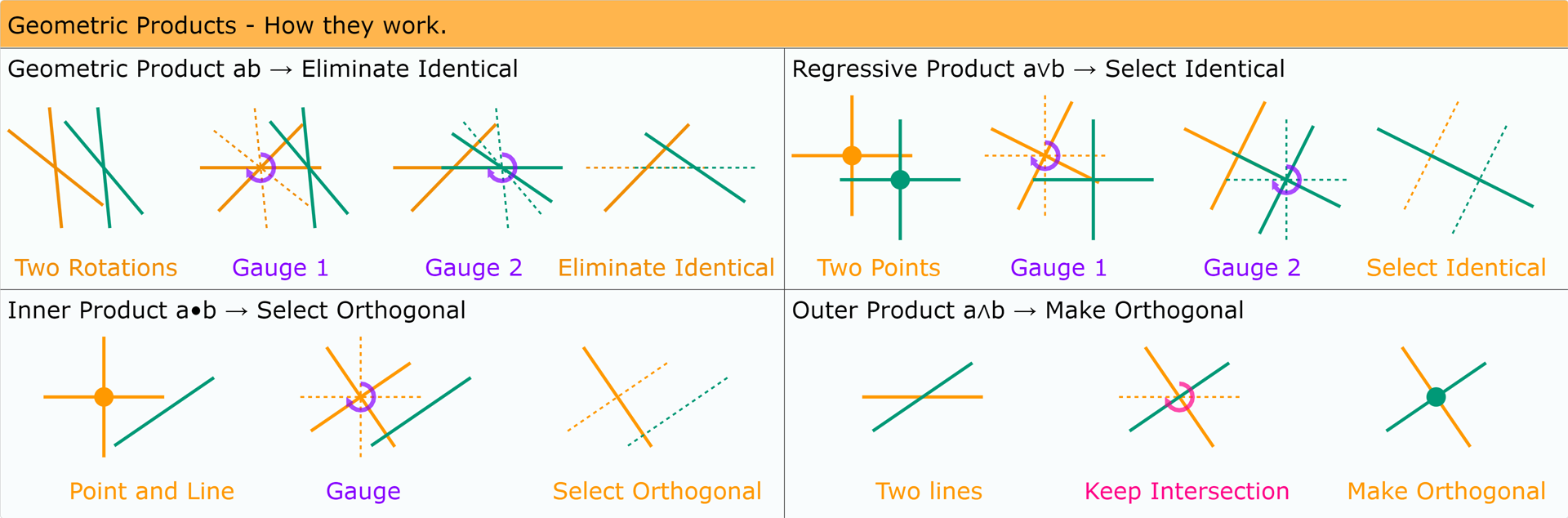
After picking the viewpoint where things look most simple, we will use the gauges to understand exactly what all of the products do geometrically.
The geometric product eliminates identical mirrors.
The First Postulate
After picking the viewpoint where things look most simple, we will use the gauges to understand exactly what all of the products do geometrically.
The geometric product eliminates identical mirrors.
The dot product eliminates parallel mirrors.
The First Postulate
After picking the viewpoint where things look most simple, we will use the gauges to understand exactly what all of the products do geometrically.
The geometric product eliminates identical mirrors.
The dot product eliminates parallel mirrors.
The regressive product keeps identical mirrors.
The outer product finds orthogonal mirrors.
Cartan-Dieudonne :
Every orthogonal transformation in an n-dimensional symmetric bilinear space can be described as the composition of at most n reflections.
The First Postulate
Tackling geometric problems :
The First Postulate
\(ab\) Geometric Product composes reflections
\(a\wedge b\) Outer Product Intersects elements
\(a\vee b\) Regressive Product joins elements
\(a\cdot b\) Dot Product rejects elements
The First Postulate
The First Postulate
Now, lets see it in action!
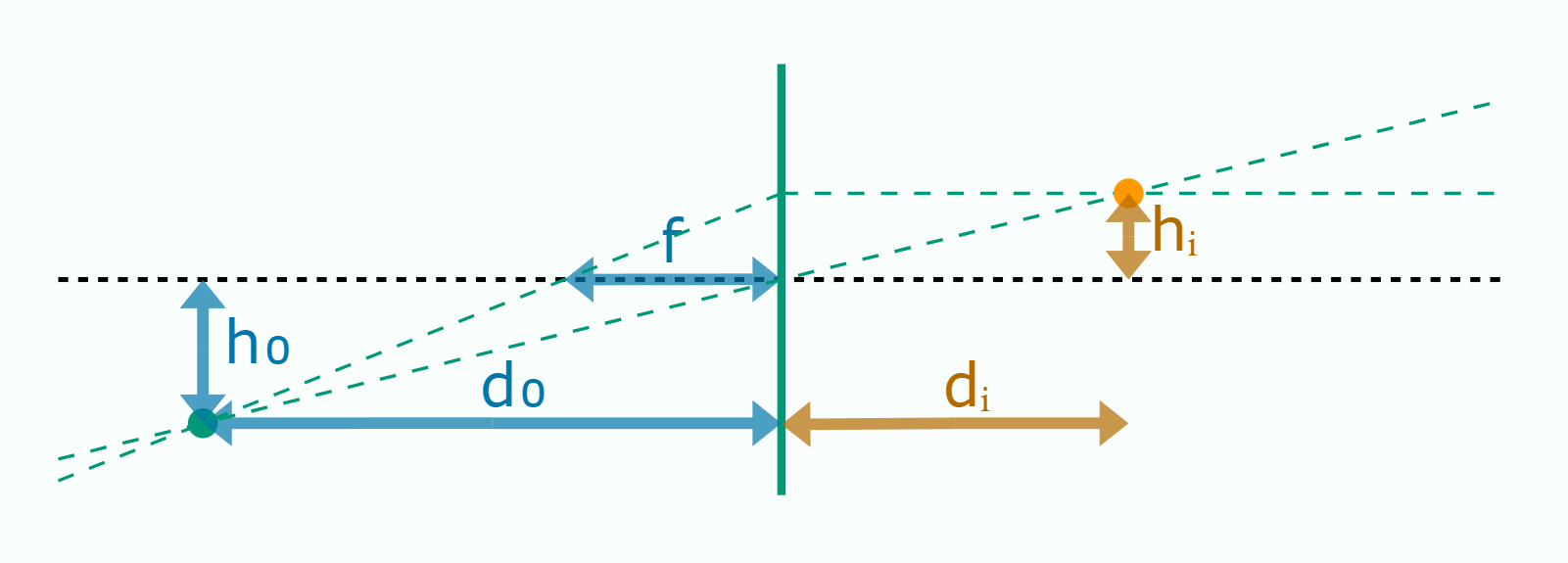
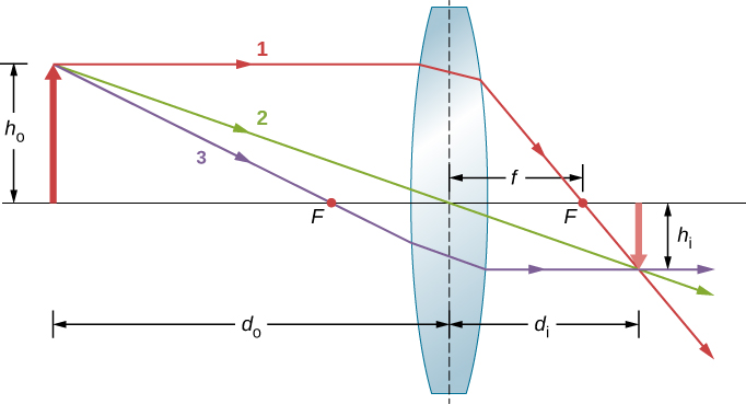
\(d_i = \big ( \frac 1 f - \frac 1 {d_0} \big )^{-1}\qquad h_i=-\frac {d_i} {d_0} h_0\)
The First Postulate
\(d_i = \big ( \frac 1 f - \frac 1 {d_0} \big )^{-1}\qquad h_i=-\frac {d_i} {d_0} h_0\)
The paraxial approximation of the thin lens equation
The First Postulate
\(d_i = \big ( \frac 1 f - \frac 1 {d_0} \big )^{-1}\qquad h_i=-\frac {d_i} {d_0} h_0\)
The paraxial approximation of the thin lens equation
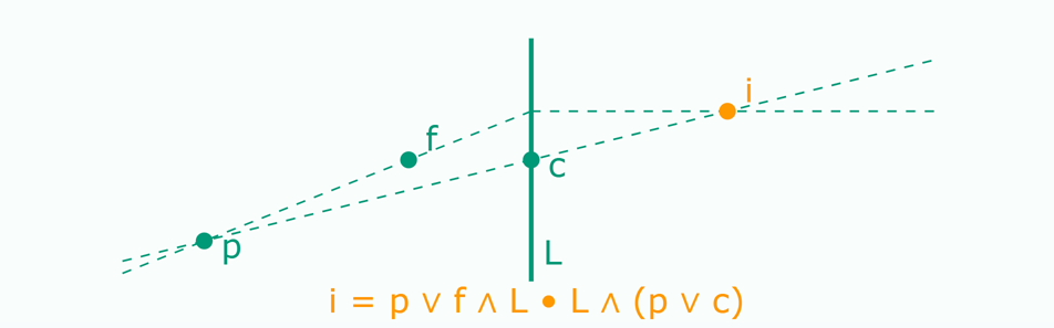
\(\vec a = \overline {\vec c - \vec f}\)
\(\vec b= \vec c - \vec p\)
\(d_0 = \vec a \cdot \vec b\)
The First Postulate
\(d_i = \big ( \frac 1 f - \frac 1 {d_0} \big )^{-1}\qquad h_i=-\frac {d_i} {d_0} h_0\)
The paraxial approximation of the thin lens equation
\((\overline {\vec c - \vec f}) \, \cdot\)
\((\vec c - \vec p)\)
\(d_0 = \)
\(h_0 = (\overline{\vec c - \vec g} )\,\cdot\,(\vec c - \vec p) \)
The First Postulate
The paraxial approximation of the thin lens equation
There are no coefficients or even ratios, and the formula can be read from left to right.
The First Postulate
The paraxial approximation of the thin lens equation
\(\vee\) = join \(\wedge\) = meet \(\bullet\) = dot
The First Postulate
The paraxial approximation of the thin lens equation
The First Postulate
Thanks!
Be sure to check Hamish's bonus talk - straight from GDC - with more real world examples!
There are still many things left uncovered, but they all build on the same simple ideas.
Itsy Bitsy Spinor
Steven De Keninck
Itsy Bitsy Spinor
| geometric product | a * b |
| meet (intersect) | a ^ b |
| join (span) | a & b |
| dot product | a | b |
| sandwich product | a >>> b |
| dual | !a |
| a point at x,y,.. | !(1e0 + x*1e1 + y*1e2 + ...) |
| a plane with eq ax + by + .. + d = 0 | a*1e1 + b*1e2 + ... + d*1e0 |
| rotate α around line L | Math.E ** ( -0.5 * α * L.Normalized ) |
Exercises at :
https://bivector.net/game2023.html
Plane-based Geometric Algebra
Plane-based Geometric Algebra
PGA
Infinity, Duality, Orientation, Forques.
Episode 3 : Revenge of Infinity
Plane-based Geometric Algebra
Infinity, Duality, Orientation, Forques.
Plane-based Geometric Algebra
PGA
Plane-based Geometric Algebra
The homogeneous model of the Euclidean plane
Text
Parallel lines intersect in points at infinity. This means intersection queries always have meaningful answers.
But infinite elements also enable duality
Plane-based Geometric Algebra
# Euclidean Lines + 1 Infinite Line = # Euclidean Points + # Infinite Points
{
{
3D Planes through origin
3D Lines through origin
\(a^* \wedge b^* = (a \vee b)^*\)
Same code to find intersection (meet) and span (join) !!
All code has two functions!
meet \(\leftrightarrow\) join
point \(\leftrightarrow\) line
Plane-based Geometric Algebra
# Euclidean Lines + 1 Infinite Line = # Euclidean Points + # Infinite Points
\(a^* \wedge b^* = (a \vee b)^*\)
translations are rotations around infinite elements !
Plane-based Geometric Algebra
Plane-based Geometric Algebra
robot arm
floor plan
robot arm
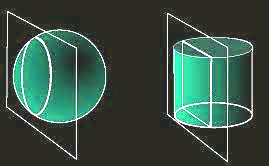
Both 2D drawings have points and lines. What happens if we go from two to three dimensions?
Duality and dimension independence
Plane-based Geometric Algebra
robot arm
floor plan
robot arm
Both 2D drawings have points and lines. What happens if we go from two to three dimensions?
Duality and dimension independence
Lines defined as 1-vectors.
Points defined as 2-vectors.
\(\rightarrow\) switch types.
Lines defined as \(d\)-\(1\) vectors.
Points defined as \(d\)-vectors.
\(\rightarrow\) stay the same type.
Plane-based Geometric Algebra
Duality and dimension independence
These can be combined - picking the correct type is key to being dimension independent.
But there is more to these types .. lets talk about orientation.
\(\rightarrow\) switch types.
\(\rightarrow\) stay the same type.
Plane-based Geometric Algebra
But there is more to these types .. lets talk about orientation.
Extrinsic
Intrinsic
MEET
JOIN
These types behave differently under reflection!
Plane-based Geometric Algebra
These concepts of two types of elements and two types of orientation are key to a dimension independent, geometric treatment of dynamics.
\(\infty\) elements, 2k-reflections
INERTIAL DUALITY
Plane-based Geometric Algebra
Forques unify linear force and angular torque.
Forques are join lines - in any number of dimensions
In the body frame, Forces and Accelerations are each others dual!!!
Forces are Join Lines - Accelerations are Meet Lines
In the body frame :
push at \(o\) = rotate around \(\infty\)
push at \(\infty\) = rotate around \(o\)
This is a tremendous simplification for the treatment of inertia.
No more need for Steiners theorem!
Fully geometric and intuitive!
Plane-based Geometric Algebra
The Geometric Overview of Rigid Body Dynamics.
FORQUE
ACCELERATION
MOMENTUM
VELOCITY
\(P=\int F\)
\(V = \int A\)
\(F=\dot P\)
\(A = \dot V\)
duality
duality
inertial
inertial
Join line through the contact point
Sum of join lines.
Meet line through the motion center
Sum of meet lines.
\((d-1)\)-vectors
\(2\)-vectors
POSITION
\(M = \int V\)
\(V = \dot M\)
Motor (\(2k\)-refl)
\(F=ma\quad \tau=mr \times F\)
\(P=mv\quad L=I\omega\)
\(F=A^\star\)
\(P=V^\star\)
Plane-based Geometric Algebra
Thanks !
Plane-based Geometric Algebra
Plane-based Geometric Algebra
PGA
Infinity, Duality, Orientation, Forques.
Episode 5 : A New Hope I
Plane-based Geometric Algebra
Plane-based Geometric Algebra
PGA
Infinity, Duality, Orientation, Forques.
Episode 5 : A new Hope I
Programming Geometric Algebra
To truly harvest the power of GA, a library that supports operator overloading is a must. (at the minimum, for prototyping)
Math Syntax
\(ab\)
\(a \wedge b\)
\(a \vee b\)
\(a \cdot b\)
\(a^*\)
\(a b \tilde a\)
Name
Geometric Product
Outer Product - Wedge
Regressive Product - Vee
Inner Product - Dot
Dual
Sandwich Product
Programming Syntax
a * b
a ^ b
a & b
a | b
!a
a >>> b
Plane-based Geometric Algebra
Infinity, Duality, Orientation, Forques.
Programming Geometric Algebra
1. Thin Lens (Paraxial Approx.)
*from phys.libretexts.org
\(d_i = (\frac {1} {f} - \frac {1} {d_0})^{-1}\)
\(h_i = - \frac {d_i}{d_0} h_0 \)
not very geometric .. but ..
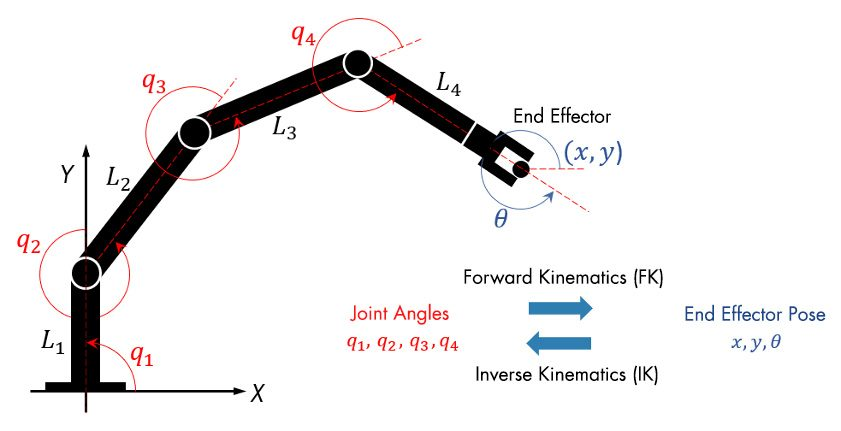
2. Inverse Kinematics
Given a thin lens, focal distance and source point calculate the position of the image point.
Given a base and target, calculate all joint orientations.
Plane-based Geometric Algebra
Infinity, Duality, Orientation, Forques.
Programming Geometric Algebra
1. Thin Lens (Paraxial Approx.)
*from phys.libretexts.org
\(d_i = (\frac {1} {f} - \frac {1} {d_0})^{-1}\)
\(h_i = - \frac {d_i}{d_0} h_0 \)
not very geometric .. but ..
Plane-based Geometric Algebra
Plane-based Geometric Algebra
PGA
Infinity, Duality, Orientation, Forques.
Episode 6 : A New Hope II
Plane-based Geometric Algebra
Plane-based Geometric Algebra
PGA
Infinity, Duality, Orientation, Forques.
Episode 6 : A new Hope II
The Geometric Overview of Rigid Body Dynamics.
FORQUE
ACCELERATION
MOMENTUM
VELOCITY
\(P=\int F\)
\(V = \int A\)
\(F=\dot P\)
\(A = \dot V\)
duality
duality
inertial
inertial
Join line through the contact point
Sum of join lines.
Meet line through the motion center
Sum of meet lines.
\((d-1)\)-vectors
\(2\)-vectors
POSITION
\(M = \int V\)
\(V = \dot M\)
Motor (\(2k\)-refl)
\(F=ma\quad \tau=mr \times F\)
\(P=mv\quad L=I\omega\)
\(F=A^\star\)
\(P=V^\star\)
Plane-based Geometric Algebra
Infinity, Duality, Orientation, Forques.
The Geometric Overview of Rigid Body Dynamics.
FORQUE
ACCELERATION
MOMENTUM
VELOCITY
\(P=\int F\)
\(V = \int A\)
\(F=\dot P\)
\(A = \dot V\)
duality
duality
inertial
inertial
Join line through the contact point
Sum of join lines.
Meet line through the motion center
Sum of meet lines.
\((d-1)\)-vectors
\(2\)-vectors
POSITION
\(M = \int V\)
\(V = \dot M\)
Motor (\(2k\)-refl)
\(F=ma\quad \tau=mr \times F\)
\(P=mv\quad L=I\omega\)
\(F=A^\star\)
\(P=V^\star\)
PGA Rigid Body Dynamics
We want it to work in n-d, so we'll need a 'rigid body' that works in 2D and 3D. We'll keep it simple and go for a square/cube.
0
1
2
3
00
01
10
11
0,0
0,1
1,0
1,1
(A^B)&(A^B-1) == 0 -> A,B differ 1 bit
By Steven De Keninck
A hands on introduction to Projective Geometric Algebra for Game and Graphics programmers.


