


Steven De Keninck PRO
Mathematical Experimentalist
Thank you all who attended - (course notes are here)
Thank you all who attended - the video will be linked when available. (course notes are here)
point
direction
line
plane
point
direction
line
plane
// construct lines
line_from_points (p1, p2)
line_from_points_and_dir (p, d)
line_from_plucker (a, b, c, d, e, f)

// construct planes
plane_from_points (p1, p2, p3)
plane_from_point_and_dirs (p, d1, d2)
plane_from_points_and_dir (p1, p2, d)
plane_from_point_and_line (p, l)
plane_from_equation (a, b, c, d)
// Intersections
intersect_line_plane (l, P)
intersect_plane_plane (P1, P2)
intersect_planes (P1, P2, P3)

// Projections
project_point_plane (p, P)
project_line_plane (l, P)
project_point_line (p, l)point
direction
line
plane
// construct lines
line_from_points (p1, p2)
line_from_points_and_dir (p, d)
line_from_plucker (a, b, c, d, e, f)

// construct planes
plane_from_points (p1, p2, p3)
plane_from_point_and_dirs (p, d1, d2)
plane_from_points_and_dir (p1, p2, d)
plane_from_point_and_line (p, l)
plane_from_equation (a, b, c, d)
// Intersections
intersect_line_plane (l, P)
intersect_plane_plane (P1, P2)
intersect_planes (P1, P2, P3)

// Projections
project_point_plane (p, P)
project_line_plane (l, P)
project_point_line (p, l)
position
rotation
point
direction
line
plane
// construct lines
line_from_points (p1, p2)
line_from_points_and_dir (p, d)
line_from_plucker (a, b, c, d, e, f)

// construct planes
plane_from_points (p1, p2, p3)
plane_from_point_and_dirs (p, d1, d2)
plane_from_points_and_dir (p1, p2, d)
plane_from_point_and_line (p, l)
plane_from_equation (a, b, c, d)
// Intersections
intersect_line_plane (l, P)
intersect_plane_plane (P1, P2)
intersect_planes (P1, P2, P3)

// Projections
project_point_plane (p, P)
project_line_plane (l, P)
project_point_line (p, l)
position
rotation
matrix
// construct transformations
mtx_translate (x, y, z)
mtx_rotate_euler (h, p, b)
mtx_rotate_axis_angle (x, y, z, a)
mtx_look_at (from, too, pole)

// apply transformations
transform_point (M, p)
transform_direction (M, d)
transform_line (M, l)
transform_plane (M, P)
point
direction
line
plane
// construct lines
line_from_points (p1, p2)
line_from_points_and_dir (p, d)
line_from_plucker (a, b, c, d, e, f)

// construct planes
plane_from_points (p1, p2, p3)
plane_from_point_and_dirs (p, d1, d2)
plane_from_points_and_dir (p1, p2, d)
plane_from_point_and_line (p, l)
plane_from_equation (a, b, c, d)
// Intersections
intersect_line_plane (l, P)
intersect_plane_plane (P1, P2)
intersect_planes (P1, P2, P3)

// Projections
project_point_plane (p, P)
project_line_plane (l, P)
project_point_line (p, l)
position
rotation
matrix
quaternion
// construct transformations
mtx_translate (x, y, z)
mtx_rotate_euler (h, p, b)
mtx_rotate_axis_angle (x, y, z, a)
mtx_look_at (from, too, pole)

// apply transformations
transform_point (M, p)
transform_direction (M, d)
transform_line (M, l)
transform_plane (M, P)
// construct transformations
quat_from_euler (h, p, b)
quat_from_axis_angle (x, y, z, a)
quat_look_at (from, too, pole)
quat_from_matrix (M)
quat_to_matrix (Q)

// apply transformations
transform_point (Q, p)
transform_line (Q, l)
transform_plane (Q, P)
velocity
force
tensor
// LA LA Land
factor_QR (M)
factor_LDL (M)
factor_SVD (M)
factor_LU (M)

.. eigenvalues ..
.. gradient descent ..
.. LMA ..
.. back prop ..
.. AD ..
point
direction
line
plane
// construct lines
line_from_points (p1, p2)
line_from_points_and_dir (p, d)
line_from_plucker (a, b, c, d, e, f)

// construct planes
plane_from_points (p1, p2, p3)
plane_from_point_and_dirs (p, d1, d2)
plane_from_points_and_dir (p1, p2, d)
plane_from_point_and_line (p, l)
plane_from_equation (a, b, c, d)
// Intersections
intersect_line_plane (l, P)
intersect_plane_plane (P1, P2)
intersect_planes (P1, P2, P3)

// Projections
project_point_plane (p, P)
project_line_plane (l, P)
project_point_line (p, l)
position
rotation
matrix
quaternion
// construct transformations
mtx_translate (x, y, z)
mtx_rotate_euler (h, p, b)
mtx_rotate_axis_angle (x, y, z, a)
mtx_look_at (from, too, pole)

// apply transformations
transform_point (M, p)
transform_direction (M, d)
transform_line (M, l)
transform_plane (M, P)
// construct transformations
quat_from_euler (h, p, b)
quat_from_axis_angle (x, y, z, a)
quat_look_at (from, too, pole)
quat_from_matrix (M)
quat_to_matrix (Q)

// apply transformations
transform_point (Q, p)
transform_line (Q, l)
transform_plane (Q, P)
velocity
force
tensor
dual quaternion
// LA LA Land
factor_QR (M)
factor_LDL (M)
factor_SVD (M)
factor_LU (M)

.. eigenvalues ..
.. gradient descent ..
.. LMA ..
.. back prop ..
.. AD ..
// and even more code..
dquat_to_matrix (DQ)
dquat_from_matrix (M)
dquat_from_direction (d)
dquat_from_euler (h, p, b)

.. meshes ..
.. computational geometry ..
.. keeps going ..point
direction
line
plane
// construct lines
line_from_points (p1, p2)
line_from_points_and_dir (p, d)
line_from_plucker (a, b, c, d, e, f)

// construct planes
plane_from_points (p1, p2, p3)
plane_from_point_and_dirs (p, d1, d2)
plane_from_points_and_dir (p1, p2, d)
plane_from_point_and_line (p, l)
plane_from_equation (a, b, c, d)
// Intersections
intersect_line_plane (l, P)
intersect_plane_plane (P1, P2)
intersect_planes (P1, P2, P3)

// Projections
project_point_plane (p, P)
project_line_plane (l, P)
project_point_line (p, l)
position
rotation
matrix
quaternion
// construct transformations
mtx_translate (x, y, z)
mtx_rotate_euler (h, p, b)
mtx_rotate_axis_angle (x, y, z, a)
mtx_look_at (from, too, pole)

// apply transformations
transform_point (M, p)
transform_direction (M, d)
transform_line (M, l)
transform_plane (M, P)
// construct transformations
quat_from_euler (h, p, b)
quat_from_axis_angle (x, y, z, a)
quat_look_at (from, too, pole)
quat_from_matrix (M)
quat_to_matrix (Q)

// apply transformations
transform_point (Q, p)
transform_line (Q, l)
transform_plane (Q, P)
velocity
force
tensor
dual quaternion
// LA LA Land
factor_QR (M)
factor_LDL (M)
factor_SVD (M)
factor_LU (M)

.. eigenvalues ..
.. gradient descent ..
.. LMA ..
.. back prop ..
.. AD ..
// and even more code..
dquat_to_matrix (DQ)
dquat_from_matrix (M)
dquat_from_direction (d)
dquat_from_euler (h, p, b)

.. meshes ..
.. computational geometry ..
.. keeps going ..
VECTOR AND MATRIX ALGEBRA
point
direction
line
plane
position
rotation
matrix
quaternion
velocity
force
dual quaternion
VECTOR AND MATRIX ALGEBRA
VECTOR
Geometric Objects are represented by choosing axes, taking measurements and writing down coefficients. Formulas produce and functions transform these measurements.
VECTOR AND MATRIX ALGEBRA
VECTOR AND MATRIX ALGEBRA
PROJECTIVE GEOMETRIC ALGEBRA
ANALYTIC GEOMETRY : VECTOR AND MATRIX ALGEBRA
ANALYTIC GEOMETRY : VECTOR AND MATRIX ALGEBRA
SYNTHETIC GEOMETRY : PROJECTIVE GEOMETRIC ALGEBRA
ANALYTIC GEOMETRY : VECTOR AND MATRIX ALGEBRA
SYNTHETIC GEOMETRY : PROJECTIVE GEOMETRIC ALGEBRA
synthetic : tools are ruler \(\rightarrow\) and compass \(\curvearrowleft\)
elements are points, lines, planes, ..
ANALYTIC GEOMETRY : VECTOR AND MATRIX ALGEBRA
SYNTHETIC GEOMETRY : PROJECTIVE GEOMETRIC ALGEBRA
synthetic : tools are ruler \(\rightarrow\) and compass \(\curvearrowleft\)
elements are points, lines, planes, ..
ANALYTIC GEOMETRY : VECTOR AND MATRIX ALGEBRA
SYNTHETIC GEOMETRY : PROJECTIVE GEOMETRIC ALGEBRA
{
{
2D
3D
.. just as in topology .. circle times circle ..
ANALYTIC GEOMETRY : VECTOR AND MATRIX ALGEBRA
SYNTHETIC GEOMETRY : PROJECTIVE GEOMETRIC ALGEBRA
{
{
2D
3D
{
4D
.. just as in topology .. circle times circle times circle ..
SYNTHETIC GEOMETRY : PROJECTIVE GEOMETRIC ALGEBRA
SYNTHETIC GEOMETRY : PROJECTIVE GEOMETRIC ALGEBRA
GEOMETRIC OBJECTS : POINTS, LINES, PLANES, ROTATIONS, TRANSLATIONS, ...
The elements of Geometry - in our case Projective Geometry
NOTE : we will work first in 2D, but in a way that will generalize to nD.
Represent Euclidean points/lines/... in n-d using an (n+1)d space.
We embed a 2D plane in a 3D space and call it the projective plane.
Represent Euclidean points/lines/... in n-d using an (n+1)d space.
We associate each projective point in 2D with a line through the origin in 3D
Represent Euclidean points/lines/... in n-d using an (n+1)d space.
Lines that do not intersect the projective plane are associated with infinite points
Represent Euclidean points/lines/... in n-d using an (n+1)d space.
#points_in_plane + #infinite_points = #lines_through_origin_in_3D
What about lines ?
Represent Euclidean points/lines/... in n-d using an (n+1)d space.
We associate each projective line in 2D with a plane through the origin in 3D
Represent Euclidean points/lines/... in n-d using an (n+1)d space.
The one plane parallel to the projective plane is associated with 1 infinite line
#points_in_plane + #infinite_points = #lines_through_origin_in_3D
#lines_in_plane + 1 = #planes_through_origin_in_3D
This works the same way in n-d and is called the Projective Map.
Represent Euclidean points/lines/... in n-d using an (n+1)d space.
The planes always intersect, and so do their corresponding lines .. even at infinity.
Represent Euclidean points/lines/... in n-d using an (n+1)d space.
The planes always intersect, and so do their corresponding lines .. even at infinity.
This means your code to intersect two lines has no exceptions, and the code that uses it has no if statements
...
// find intersection
  var point = intersect_lines(line1, line2)

// always a valid result. (possibly infinite point).
// no checking - just use it !
...
What happens when you rotate around an infinite point ?
Represent Euclidean points/lines/... in n-d using an (n+1)d space.
#points_in_plane + #infinite_points = #lines_through_origin_in_3D
#lines_in_plane + 1 = #planes_through_origin_in_3D
#lines_through_origin_in_3D = #planes_through_origin_in_3D
each 3D line is orthogonal to exactly one 3D plane so we also have :
that also means the same amount of projective points and lines !
so we can relate projective lines and planes leading to Duality
Represent Euclidean points/lines/... in n-d using an (n+1)d space.
JOIN of two points is dual to MEET of their two dual lines
DUALITY : associate each projective point with one projective line
Represent Euclidean points/lines/... in n-d using an (n+1)d space.
JOIN of two points is dual to MEET of two lines
line is collection of points on it
point is collection of lines through it
Represent Euclidean points/lines/... in n-d using an (n+1)d space.
JOIN of two points is dual to MEET of two lines
your code to intersect two lines can also be used to join two points.
function join_points(point1,point2) {
  // dualize input points
  var line1 = dual(point1);
  var line2 = dual(point2);
  // find intersection point.
  var intersection_point = intersect_lines(line1, line2);
  // return the dual line of this point
  return dual(intersection_point);
}
point
lies on
line
intersect
Works for all your functions !!!!!
Rotate around \(\infty\) = Push at CoG
Rotate around CoG = Push at \(\infty\)
|
|
|---|
Rotate around CoG
Rotate around \(\infty\)
Push at \(\infty\)
Push at CoG
ALL FORCES ARE LINEAR, ALSO THE ANGULAR ONES, BOTH IN 2D AND 3D !
lines are special !
\(\curvearrowleft\)
\(\curvearrowleft\)
\(\uparrow\)
\(\uparrow\)
\(\curvearrowleft\)
\(\infty\)
\(\infty \)
\(\uparrow\)
Represent Euclidean points/lines/... in n-d using an (n+1)d space.
Where are the formula's and numbers ? We have changed our difficult to write down arbitrary points and lines to slightly less difficult to write down entities through the origin. For lines through the origin we can use VECTORS, but lets think some more on the writing down .. enter Algebra.
What picture do you get when you see this equation ?
What picture do you get when you see this equation ?
| ax² = bx | ax² = c |
| bx = c | ax² + bx = c |
| ax² + c = bx | bx + c = ax² |
Al-Khwarizmi's six problems
Today, one problem :
What was Al-Khwarizmi missing ?
| ax² = bx | ax² = c |
| bx = c | ax² + bx = c |
| ax² + c = bx | bx + c = ax² |
Al-Khwarizmi's six problems
Today, one problem :
What was Al-Khwarizmi missing ?
no negative numbers, no zero
more numbers, less formulas, less code.
What was Al-Khwarizmi missing ?
zero negative numbers
what are these crazy un-natural numbers ?
\(\rightarrow\) They're not natural numbers !
\(\rightarrow\) Yet they square to a natural number ??
What was Al-Khwarizmi missing ?
zero negative numbers
maybe other numbers were hiding ?
What was Al-Khwarizmi missing ?
zero negative numbers
maybe other numbers were hiding ?
What was Al-Khwarizmi missing ?
zero negative numbers
maybe other numbers were hiding ?
What was Al-Khwarizmi missing ?
zero negative numbers
maybe other numbers were hiding ?
What was Al-Khwarizmi missing ?
zero negative numbers
maybe other numbers were hiding ?
What was Al-Khwarizmi missing ?
zero negative numbers
maybe other numbers were hiding ?
What was Al-Khwarizmi missing ?
zero negative numbers
maybe other numbers were hiding ?
What was Al-Khwarizmi missing ?
zero negative numbers
maybe other numbers were hiding ?
What was Al-Khwarizmi missing ?
zero negative numbers
maybe other numbers were hiding ?
BASIC INSIGHT : 0D,1D,2D,... numbers behave differently
THE GEOMETRIC NUMBERS
these are of course the complex, hyperbolic and dual numbers. So why call them geometric numbers ? lets find out ..
Addition and Scalar multiplication are trivial :
a lemon plus a lemon is almost always two lemons.
Addition and Scalar multiplication are trivial :
a lemon plus a lemon is almost always two lemons.
But what about multiplication ? we'll just try ..
We add \(\mathbf e_-\) to our bag of numbers. Each element in it is now of the form (a + b\(\mathbf e_-\)).
We add \(\mathbf e_-\) to our bag of numbers. Each element in it is now of the form (a + b\(\mathbf e_-\)).
So, nothing special to remember ! No new multiplication, just a new element in the bag.
Easy to calculate - but what does it DO ?
Easy to calculate - but what do they DO ?
Elements that square to -1 related to ROTATIONS
\(\hookrightarrow\) this means \(-e_-\) is the inverse of \(e_-\)
Easy to calculate - but what do they DO ?
Elements that square to 0 related to TRANSLATIONS
\(\rightarrow (1+\epsilon)^{1.5}\) ?
ROTATIONS
HYPERBOLIC ROTATIONS
TRANSLATIONS
ROTATIONS
TRANSLATIONS
Also, we want translations and rotations in one bag. But first - we solve the "smooth" and "weird 1+" problems.
HYPERBOLIC ROTATIONS
With \(e_-^n\) where \(n \in \mathbb N\) we can rotate in steps. What about \(e_-^x\) with \(x \in \mathbb R\) ?
\({(4^2)}^2 = (4*4)^2 = (4*4)*(4*4) = 4^{2*2} = 4^4\)
\(4^x = {(2^2)}^x = 2^{2x}\)
\(a^x = {(b^{\alpha})}^x = b^{\alpha x}\)
\(\hookrightarrow\)
All exponential functions are the same, with x scaled by some constant \(\alpha\).
So if we can calculate one smooth \(a^x\) with \(x \in \mathbb R\), we're done.
\(e^x = 1 + \frac x 1 + \frac {x^2} {2*1} + \frac {x^3} {3*2*1} + ...\)
power can be ANYTHING
powers \(\in \mathbb N\)
So, if you see \(e^x\), the \(e\) ONLY tells you its an exponential function, the \(x\) has all the information. With our new numbers, \(e^{\alpha e_-}\) are thus rotations and \(e^{\alpha e_0}\) are translations.
\(e^{\alpha \mathbf e_-}=\sum \limits_{n=0}^\infty \cfrac {(\alpha \mathbf e_-)^n} {n!} = \cos \alpha + \sin \alpha \mathbf e_-\)
\(\rightarrow\) Exponentiate \(\alpha \mathbf e_-\) to get a rotation (these are our smooth rotations)
\(e^{\alpha \mathbf e_0}=\sum \limits_{n=0}^\infty \cfrac {(\alpha \mathbf e_0)^n} {n!} = 1 + \alpha \mathbf e_0\)
\(\rightarrow\) Exponentiate \(\alpha \mathbf e_0\) to get a translation. (this is that weird \(+1\))
With \(e_-^n\) where \(n \in \mathbb N\) we can rotate in steps. What about \(e_-^x\) with \(x \in \mathbb R\) ?
\(\vec{x} = a\mathbf e_1 + b\mathbf e_2\)
THE CONTRACTION AXIOM :
\(\vec{x} = a\mathbf e_1 + b\mathbf e_2\)
By the contraction axiom, any such vector must square to a real number :
\((a\mathbf e_1 + b\mathbf e_2)^2 = a^2\mathbf e_1^2 + ab\mathbf e_1\mathbf e_2 + ba\mathbf e_2\mathbf e_1 + b^2\mathbf e_2^2\)
THE CONTRACTION AXIOM :
\(\vec{x} = a\mathbf e_1 + b\mathbf e_2\)
By the contraction axiom, any such vector must square to a real number :
\((a\mathbf e_1 + b\mathbf e_2)^2 = a^2\mathbf e_1^2 + ab\mathbf e_1\mathbf e_2 + ba\mathbf e_2\mathbf e_1 + b^2\mathbf e_2^2\)
Since \(a^2\mathbf e_1^2,b^2\mathbf e_2^2\) are both scalar, and \(\mathbf e_1\mathbf e_2\) and \(\mathbf e_2\mathbf e_1\) can not be simplified :
\(ab\mathbf e_1\mathbf e_2 + ba\mathbf e_2\mathbf e_1 = 0\)
\(\leftrightarrow \mathbf e_1\mathbf e_2 = -\mathbf e_2\mathbf e_1\)
THE CONTRACTION AXIOM :
\(\mathbf e_i\mathbf e_j = -\mathbf e_j\mathbf e_i\)
\(\mathbf e_i \notin \mathbb R\)
\(\mathbf e_i^2 \in \mathbb R\)
\(\mathbf e_i\mathbf e_j = \mathbf e_{ij}\)
A general element of our GA is called a multivector and is the sum of a scalar, vector, bivector, ...
So, we start with two elements \(\mathbf e_1, \mathbf e_2\), and through multiplication we get another new element, \(\mathbf e_{12}\). It is the plane our two vectors lie in.
\(\mathbb R_{2,0,0} :\)
\(\mathbb R\)
\(\mathbf e_1,\mathbf e_2\)
\(\mathbf e_{12}\)
\(\rightarrow\) 0-dimensional "scalar"
\(\rightarrow\) 1-dimensional "vector"
\(\rightarrow\) 2-dimensional "bivector"
a vector is a 1D oriented quantity. (line)
a bivector is a 2D oriented quantity. (plane)
a trivector is a 3D oriented quantity (volume)
in practice, only two calculation rules ! \(e_ie_i = \{+1,-1,0\},\quad e_ie_j = -e_je_i\)
Let's try a few examples, with two basis vectors, \(\mathbf e_1,\mathbf e_2\), both square to +1
\(3\mathbf e_1 2\mathbf e_1 = 6\)
\(3\mathbf e_1 2\mathbf e_2 = 6 \mathbf e_1\mathbf e_2 = 6 \mathbf e_{12}\)
\((3\mathbf e_1 + \mathbf e_2) \mathbf e_2 = 3\mathbf e_{12} + 1\)
\(\mathbf e_2 \mathbf e_{12} = \mathbf e_2 \mathbf e_1 \mathbf e_2 = - \mathbf e_1 \mathbf e_2 \mathbf e_2 = - \mathbf e_1\)
\(\mathbf e_{12} \mathbf e_{12} = \mathbf e_1 \mathbf e_2 \mathbf e_1 \mathbf e_2 = - \mathbf e_1 \mathbf e_1 \mathbf e_2 \mathbf e_2 = -1 \)
bivector rotates !
We'll want more elements in the same bag, and names will get confusing, so let's first introduce some notation :
\(\mathbb R_{positive,negative,zero}\)
\(\mathbb R_{0,1,0}\,\rightarrow\) one extra element that squares to \(-1\)
\(\mathbb R_{0,0,1}\,\rightarrow\) one extra element that squares to \(0\)
\(\mathbb R_{9,6,0}\,\rightarrow\) nine extra element that square to \(1\)
and six extra elements that square to \(-1\)
These elements are called generators, and are typically written \(\mathbf e_0, \mathbf e_1, \mathbf e_2, ...\)
so, only two calculation rules ! \(e_ie_i = \{+1,-1,0\},\quad e_ie_j = -e_je_i\)
square any generator, replace with metric
swap two generators, change sign
product of any two vectors in \(\mathbb R_{3,0,0}\) :
\((a_1\mathbf e_1 + a_2\mathbf e_2 + a_3\mathbf e_3)(b_1\mathbf e_1 + b_2\mathbf e_2 + b_3\mathbf e_3) = \)
\(a_1b_1 + a_2b_2 + a_3b_3\\+ (a_1b_2-a_2b_1)\mathbf e_{12} + (a_1b_3-a_3b_1)\mathbf e_{13} + (a_2b_3-a_3b_2)\mathbf e_{23}\)
The product of two VECTORS is a SCALAR + BIVECTOR
\(a*b\) \(=\) \(a \cdot b\) \(+\) \(a \wedge b\)
geometric product
inner product (dot)
outer product (wedge, 'cross')
\(a*b\) \(=\) \(a \cdot b\) \(+\) \(a \times b\)
\(\mathbb R_{3,0,0}\)
Scalars + Bivectors = QUATERNIONS
RECAP :
\(ab\) = geometric product
\(a \cdot b\) = inner product
\(a \wedge b\) = outer product
\(a^*\) = dual of \(a\)
\(a \vee b\) = \((a^* \wedge b^*)^*\)
\(=\) regressive product
\(ab\) = geometric product
\(a \cdot b\) = inner product
\(a \wedge b\) = outer product
\(a^*\) = dual of \(a\)
\(a \vee b\) = \((a^* \wedge b^*)^*\)
\(=\) regressive product
We can now pick the Algebra that best fits our problem. For our current problem of computer geometry, we need it to store points, directions, lines, planes, translations and rotations.
We are now ready to create the bag we need for 2D PGA - The projective plane
We need a 1-up model, so start with three basis vectors :
\(\mathbf e_0, \mathbf e_1, \mathbf e_2 \)
where \(\mathbf e_0\) is the projective dimension. This results
in three bivectors \(\mathbf e_{01}, \mathbf e_{20}, \mathbf e_{12} \) and one trivector \(\mathbf e_{012}\)
remembering that we need bivectors for isometries, we consider the metric for \(\mathbf e_0\)
\({\mathbf e_0}^2 = +1 \quad \rightarrow \quad {\mathbf e_{01}}^2=-1, {\mathbf e_{20}}^2=-1, {\mathbf e_{12}}^2 = -1\)
\({\mathbf e_0}^2 = -1 \quad \rightarrow \quad {\mathbf e_{01}}^2=+1, {\mathbf e_{20}}^2=+1, {\mathbf e_{12}}^2 = -1\)
\({\mathbf e_0}^2 = 0 \quad \rightarrow \quad {\mathbf e_{01}}^2=0, {\mathbf e_{20}}^2=0, {\mathbf e_{12}}^2 = -1\)
Only with \(\mathbf e_0^2=0\) we get the two translations and one rotation we need for isometries in the 2D Euclidean plane.
\(\rightarrow\) elliptic
\(\rightarrow\) hyperbolic
\(\rightarrow\) Euclidean
\(\mathbb R^*_{2,0,1}\)
Scalars + Bivectors = Translate + Rotate
We are now ready to create the bag we need for 2D PGA - The projective plane
| 1 | e0 | e1 | e2 | e01 | e20 | e12 | e012 |
|---|
vector
bivector
scalar
trivec
projective LINES
projective POINTS
| +1 | 0 | +1 | +1 | 0 | 0 | -1 | 0 |
|---|
Unifies TRANSFORMATION and ELEMENT !! \(e^\mathbf x =\) rotation around \(\mathbf x\) !!
also in 3D ! "Plane based GA"
We are now ready to create the bag we need for 2D PGA - The projective plane
| 1 | e0 | e1 | e2 | e01 | e20 | e12 | e012 |
|---|
vector
bivector
scalar
trivec
projective LINES
projective POINTS
Point at (x,y) :
Line between points \(p_1, p_2\) :
Line with equation \(a\mathbf x + b\mathbf y + c= 0\) :
Intersect lines \(\ell_1, \ell_2\) :
Rotation of \(\alpha\) around point \(p\) :
Translate \(\alpha\) with infinite point \(p\) :
Angle between lines \(\ell_1, \ell_2\) :
Project point on line :
\(x\mathbf e_{20} + y\mathbf e_{01} + \mathbf e_{12}\)
\(p_1 \vee p_2\)
\(a\mathbf e_1 + b\mathbf e_2 + c\mathbf e_0\)
\(\ell_1 \wedge \ell_2\)
\(e^{\alpha p}\)
\(e^{\alpha p}\)
\(\cos^{-1}(\ell_1 \cdot \ell_2)\)
\( (\ell \cdot p) \ell\)
| +1 | 0 | +1 | +1 | 0 | 0 | -1 | 0 |
|---|
Now that we can multiply points and lines, lets look at some interesting products :
The regressive product \(\vee\)
JOINS points into lines
\(\ell=P_1 \vee P_2\\\,\,\,\,\,\,\,\,\,\,\,= (P_1^* \wedge P_2^*)^*\)
The outer product \(\wedge\)
MEETS lines in points
\(P=\ell_1 \wedge \ell_2\)
Now that we can multiply points and lines, lets look at some interesting products :
\(\ell\) = line (vector)
\(P\) = point (bivector)
\(\ell P\) = line through \(P, \perp\) to \(\ell\)
\(\ell P\ell\) = reflection of \(P\) in \(\ell\)
\(P\ell P\) = reflection of \(\ell\) in \(P\)
\((\ell \cdot P)\ell\) = projection of \(P\) on \(\ell\)
\((P \cdot \ell)P\) = projection of \(\ell\) on \(P\)
Now that we can multiply points and lines, lets look at some interesting products :
\(\ell_1 P\ell_1\) = reflection of \(P\) in \(\ell_1\)
\(\ell_2\ell_1 P\ell_1\ell_2\) = reflection of \(P\) in \(\ell_1\) then \(\ell_2\)
two reflections in lines (vectors)
= rotation around intersection point (bivector)
Just like the quaternions, a transformation \(m = \ell_1\ell_2\) is applied on an element \(\bf x\) using the "sandwich product" :
\( m \mathbf x \tilde m\)
where \(\tilde m\) is the reverse of \(m\) (here \(\tilde m =\ell_2 \ell_1\))
Free of coordinates, chirality and insensible representations for rotations,
many algorithms trivialize. Inverse Kinematics in 4 lines, no if statements :
// &   = JOIN, regressive product
// >>> = SANDWICH

// c is array of PGA points in ik chain

function solveIK( c, target ) {
    for (j=0;j<4; j++) {
    // Set end of chain to target.
      c[l-1] = target;

    // Run backwards, restore the lengths
      for (i=l-2; i>0; i--)
        c[i] = translator(c[i]&c[i+1],-d) >>> c[i+1];

    // Run forwards, restore lengths again
      for (i=1; i<l; i++)
        c[i] = translator(c[i-1]&c[i],-d) >>> c[i-1];
    }
}
Free of coordinates, chirality and insensible representations for rotations,
many algorithms trivialize. Seperating Axis test in 11 lines of code :
// Seperating Axis test
// a,b are arrays of points

function sat(a,b) {
// Collect potential axis candidates
  var e=[], da=[], db=[], i, al=a.length, bl=b.length;
  for (i=0; i<al; i++) e[i]=(a[i]&a[(i+1)%al]).Normalized;
  for (i=0; i<bl; i++) e[i+al]=(b[i]&b[(i+1)%bl]).Normalized;
// Testing a single axis
  var check=(axis)=>{
    for (var i=0; i<al; i++) da[i]=(a[i]^axis).e012;
    for (var i=0; i<bl; i++) db[i]=(b[i]^axis).e012;
    return (Math.min(...da)>Math.max(...db))
         ||(Math.min(...db)>Math.max(...da));
  }
// Test all edges. Return the separating axis if found.
  for (i=0; i<e.length; i++) if (check(e[i])) return e[i];
}
It is all exactly the same in 3D, just some more elements :
It is all exactly the same in 3D, just some more elements :
| 1 | e0 | e1 | e2 | e3 | e01 | e02 | e03 |
|---|
Point at (x,y,z) :
Line between points \(P_1, P_2\) :
Plane with equation \(a\mathbf x + b\mathbf y + c\mathbf z + d = 0\) :
Intersect planes \(p_1, p_2\) :
Rotation of \(\alpha\) around line \(L\) :
Translate \(\alpha\) with infinite line \(L\) :
Angle between planes \(p_1, p_2\) :
Project point on plane :
\(x\mathbf e_{023} + y\mathbf e_{013} + z\mathbf e_{012} + \mathbf e_{123}\)
\(P_1 \vee P_2\)
\(a\mathbf e_1 + b\mathbf e_2 + c\mathbf e_3 + d\mathbf e_0\)
\(p_1 \wedge p_2\)
\(e^{\alpha L}\)
\(e^{\alpha L}\)
\(\cos^{-1}(p_1 \cdot p_2)\)
\( (p \cdot P) p\)
| +1 | 0 | +1 | +1 | +1 | 0 | 0 | 0 |
|---|
| e12 | e13 | e23 | e012 | e013 | e023 | e123 | e0123 |
|---|
| scalar | vector | bivector | trivector | PSS |
|---|
| PROJECTIVE PLANES | PROJECTIVE LINES | PROJECTIVE POINTS |
|---|
| -1 | -1 | -1 | 0 | 0 | 0 | -1 | 0 |
|---|
The regressive product \(\vee\) JOINS points or lines in lines or planes
\(\ell=P_1 \vee P_2\)
\(p = P_1 \vee P_2 \vee P_3 \)
The outer product \(\wedge\) MEETS
planes or lines in lines or points
\(\ell=p_1 \wedge p_2\)
\(P = p_1 \wedge p_2 \wedge p_3 \)
All incidence relations trivially work, and algebraic expressions with points, lines and planes can be simplified like any other.
The PGA motors are isomorphic to the Dual Quaternions. They can be trivially interpolated, and no matrix conversions are needed.
// >>> = SANDWICH product.
// B1, W1 = Bone1 motor and its weight
// B2, W2 = Bone2 motor and its weight
// W1 + W2 = 1

if (Dual_Quaternion) {

 // Blend motors, apply to point.
 points[i] = (w1 * b1 + w2 * b2).Normalized >>> points_orig[i];

} else {

 // Apply both motors, blend result.
 points[i] = w1 * (b1 >>> points_orig[i]) +
             w2 * (b2 >>> points_orig[i]);

}Like our torus example in the introduction, motor orbits can be used to create a wide variety of shapes using constructions known from topology
// A segment is a translation.
  SEGMENT = (BV)=>x=>1+x*BV,
// A circle as the product of a rotation and a translation.
  CIRCLE = (BV,r)=>x=>E**(PI*x*BV)*(1+r*1e01),
// A plane is the product of two segments.
  PLANE = (a,b)=>SEGMENT(a)*SEGMENT(b),
// A sphere as a product of a degenerate circle and a circle.
  SPHERE  = (r)=>CIRCLE(1e12,0)*CIRCLE(1e13,r),
// A torus as the product of two circles
  TORUS  = (r1,r2)=>CIRCLE(1e12,r1)*CIRCLE(1e13,r2),
// A cylinder is the product of a segment and a circle
  CYLINDER = (r,h)=>CIRCLE(1e12,r)*SEGMENT(h*1e03),
// A disk is the product of a segment and (degenerate) circle
  DISK = (r)=>CIRCLE(1e13,0)*SEGMENT(1e01*r),
// and so is a cone ..
CONE = (r,h)=>CIRCLE(1e12,0)*SEGMENT(1e01*r+1e03*h);Exception free incidence calculations have many obvious applications.
// recalculate the slice. (cuts of all polies with cutplane)
var contour=[];

faces.forEach((x,i)=>{
  var [f,e1,e2,e3]=facedata[i], res=[],
      l=(f^cut), p1=(l^e1), p2=(l^e2), p3=(l^e3),
      p12=(p1&e2).s>=0,
      p13=(p1&e3).s>=0,
      p23=(e3&p2).s>=0;
  if (p1.e123 && (p12 == p13)) res.push(p1);
  if (p2.e123 && (p12 == p23)) res.push(p2);
  if (p3.e123 && (p13 != p23)) res.push(p3);
  if (res.length==2) contour.push(res);
})
PGA points, lines and planes are excellent for mesh vertices, edges and faces.
Edges \(E\) and Faces \(F\)
\(E_i = \widehat{P_1} \vee \widehat{P_2}\quad\quad\quad F_i = \widehat{P_1} \vee \widehat{P_2} \vee \widehat{P_3}\)
Polygon circumference \(c\) and area \(a\):
\(c=\sum\lVert E_i\rVert\quad a=\frac 1 2 \lVert \sum E_i \rVert_\infty\)
Mesh area \(a\) and volume \(v\)
\(a=\frac 1 2 \sum\lVert F_i\rVert\quad v=\frac 1 3 \lVert \sum F_i \rVert_\infty\)
PGA points, lines and planes are excellent for mesh vertices, edges and faces.
Edges \(E\) and Faces \(F\)
\(E_i = \widehat{P_1} \vee \widehat{P_2}\quad\quad\quad F_i = \widehat{P_1} \vee \widehat{P_2} \vee \widehat{P_3}\)
for DDG, similar simple formulas :
\(\Omega_j = 2\pi - \sum \cos^{-1}({\widehat{E}_i\cdot \widehat{E}_{i+1}})\)
\(2\pi\chi = \sum \Omega_j\)
note - no edge vectors needed ..
Unification of elements and transformations, makes implementing origami as easy as folding paper.
// The first three Huzita-Hatori axioms

// The fold between p1 and p2
  var Ori1 = (p1,p2)=>p1 & p2 & 1e023;

// fold p1 onto p2
  var Ori2 = (p1,p2)=>(p1&p2)<<(p1+p2).Normalized;

// fold line l1 onto line l2
  var Ori3 = (l1,l2,flag)=>{
    l1=l1.Normalized;
    l2=l2.Normalized;
    return flag==0?(l1+l2)&1e023:((l1+l2)<<(l1&1e023^l2))
  };
point
direction
line
plane
// construct lines
line_from_points (p1, p2)           = p1&p2
line_from_points_and_dir (p, d)     = p&(p+d)


// construct planes
plane_from_points (p1,p2,p3)        = p1&p2&p3
plane_from_point_and_dirs (p,d1,d2) = p&(p+d1)&(p+d2)
plane_from_points_and_dir (p1,p2,d) = p1&p2&(p1+d)
plane_from_point_and_line (p,l)     = p&l
plane_from_equation (a,b,c,d)       = ae1+be2+ce3-de0
// Intersections
intersect_line_plane (l, P) = l^P
intersect_plane_plane (P1, P2) = P1^P2
intersect_planes (P1, P2, P3) = P1^P2^P3
// Projections
project_point_plane (p, P) = P|p*P
project_line_plane (l, P) = P|l*P
project_point_line (p, l) = l|p*lposition
rotation
matrix
quaternion
// construct transformations -> motors, not matrices !
translate (x,y,z)             = E**(x*e01+y*e02+z*e03)
rotate_euler (h,p,b)          = E**(b*e12)*E**(p*e23)*E**(h*e13)
rotate_axis_angle (x,y,z,a)   = E**(a*x*e23+a*y*e13+a*z*e12)
look_at (from,too,pole)       = (1 + (e1-from)*(to-from))

// apply transformations -> note : all the same..
transform_point (M, p)        = M*p*~M
transform_direction (M, d)    = M*d*~M
transform_line (M, l)         = M*l*~M
transform_plane (M, P)        = M*P*~M
// construct transformations
quat_from_euler (h, p, b)
quat_from_axis_angle (x, y, z, a)
quat_look_at (from, too, pole)
quat_from_matrix (M)
quat_to_matrix (Q)

// apply transformations
transform_point (Q, p)
transform_line (Q, l)
transform_plane (Q, P)
Same as opening but now in PGA - implementation is shorter than function names !
no coordinates - no chirality - no gimbal lock - no conversions
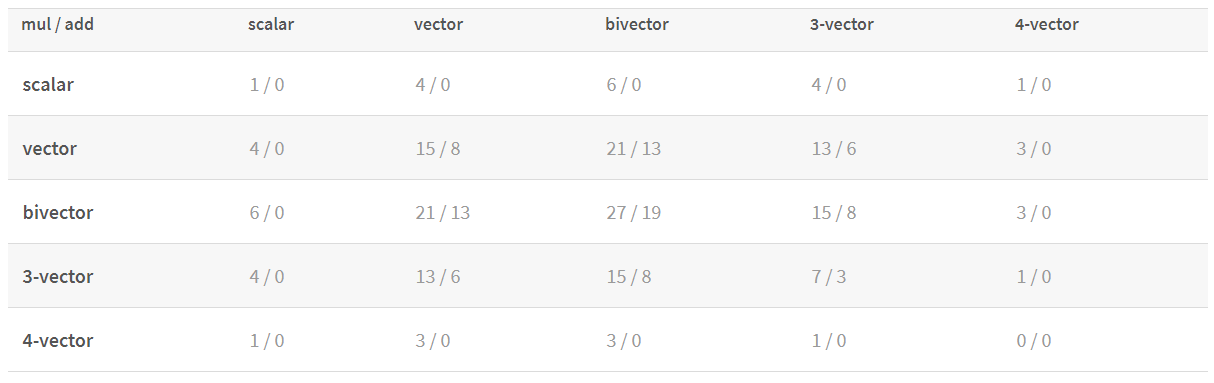
4x4 matrix multiplication : 64 multiplications, 48 additions, 16 floats
PGA motor multiplication : 48 multiplications, 40 additions, 8 floats
with a similar picture for the other elements :
Reference implementations for C++, C#, Python, Rust and javascript are available at :
also the place for the cheat-sheets, course notes, and the home of our forum.
By Steven De Keninck
SIGGRAPH2019 - gensub345b - Geometric Algebra for Computer Graphics


