


Erik Jansson
WASP and KAW postdoctoral fellow in the Cambridge Image Analysis Group and CRA at Wolfson College.
A. Bonito, D. Guignard, and W. Lei, Numerical approximation of Gaussian random fields on
closed surfaces, Computational and Applied Mathematics. In press (2024)
Dziuk, G., and Elliott, C. M., Finite element methods for surface PDEs. Acta Num., 22:289–396, 2013.
H. Fujita and T. Suzuki, Evolution problems, Handbook of Numerical Analysis, pp. 789–928,
Whittle, P., Stochastic processes in several dimensions. Bull. Inst. Int. Stat., 40:974–994, 1963.
asdasdasd
https://arxiv.org//2406.08185
D. Boffi, Finite element approximation of eigenvalue problems, Acta Numerica, pp. 1-120 (2010).
A. Yagi, Abstract Parabolic Evolution Equations and Their Applications, Springer Monographs in Mathematics, Springer, Berlin, 2010.
Bolin, D., Kirchner, K., Kovács, M., Numerical solution of fractional elliptic stochastic PDEs with spatial white noise, IMA J. Numer. Anal., 40(2):1051–1073, 2020
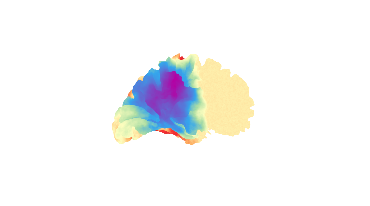
The SPDE view: Consider GRFs that are solutions to elliptic stochastic partial differential equations on manifolds:
In this talk: Manifolds = compact, boundary–less oriented embedded surfaces or curves in \(\mathbb{R}^3\) or \(\mathbb{R}^2\)
Elliptic differential operator
White noise
Two questions:
Sampling
Statistics
Elliptic differential operator
White noise
Two questions:
Sampling
Statistics
In this talk: Manifolds = compact, boundary–less oriented embedded surfaces or curves in \(\mathbb{R}^3\) or \(\mathbb{R}^2\)
The SPDE view: Consider GRFs that are solutions to elliptic stochastic partial differential equations on manifolds:
Elliptic differential operator
White noise
Two questions:
Computation
Statistics
In this talk: Manifolds = compact, boundary–less oriented embedded surfaces or curves in \(\mathbb{R}^3\) or \(\mathbb{R}^2\)
The SPDE view: Consider GRFs that are solutions to elliptic stochastic partial differential equations on manifolds:
Eigenpairs of \( \mathcal{L} \): \((\lambda_i,e_i)\)
+ Conditions
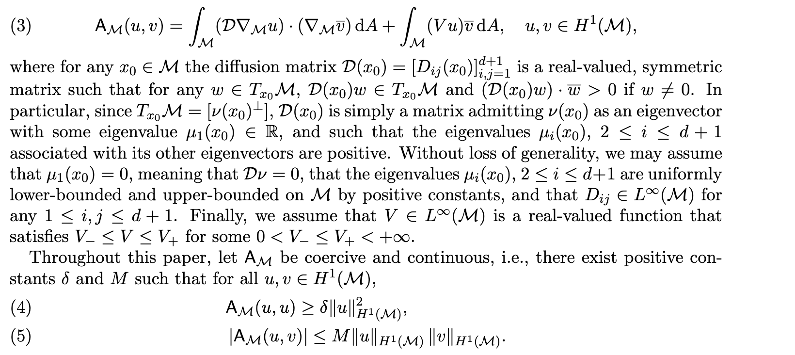
\(\mathsf A_\mathcal{M}\) defines elliptic operator \(\mathcal L\)
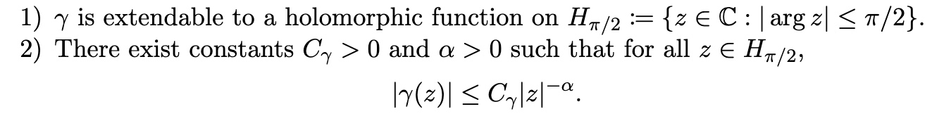
\(\gamma\colon\mathbb{R}_+ \to \mathbb{R}\) is a function satisfying sufficient decay properties (plus more)
formally
Some examples
5
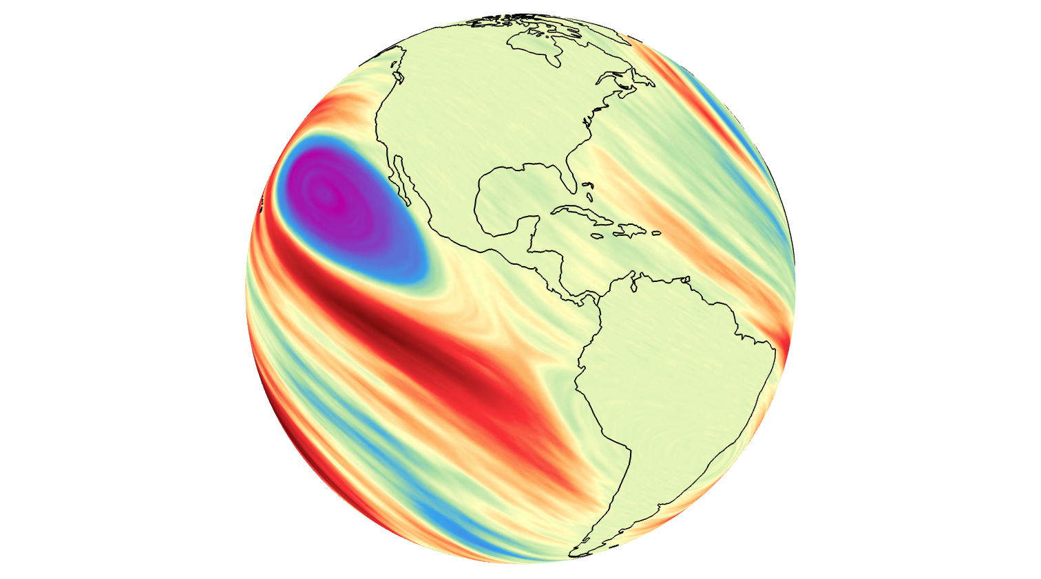
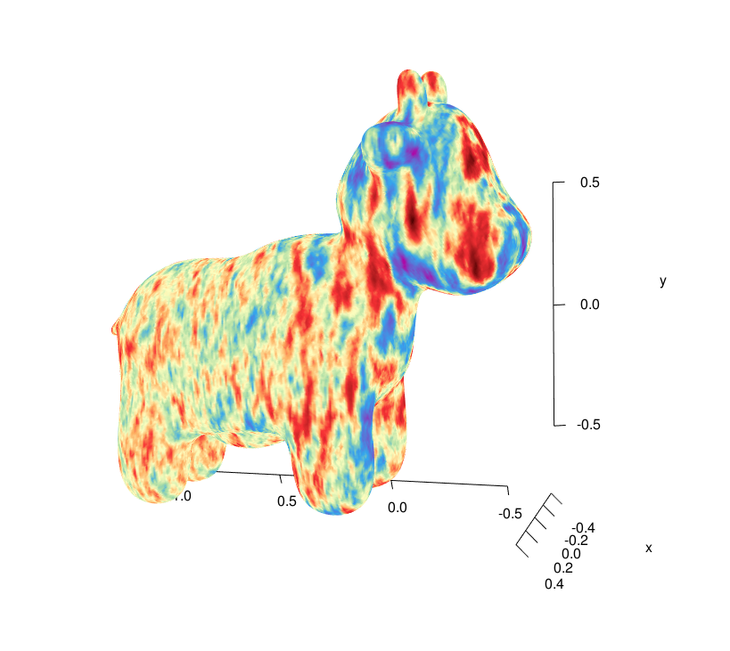
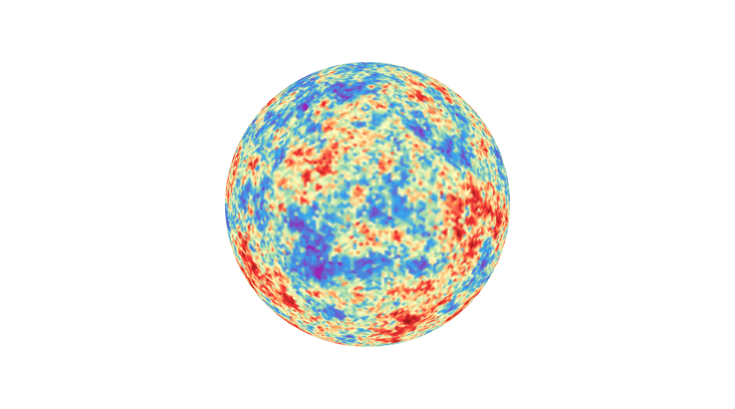
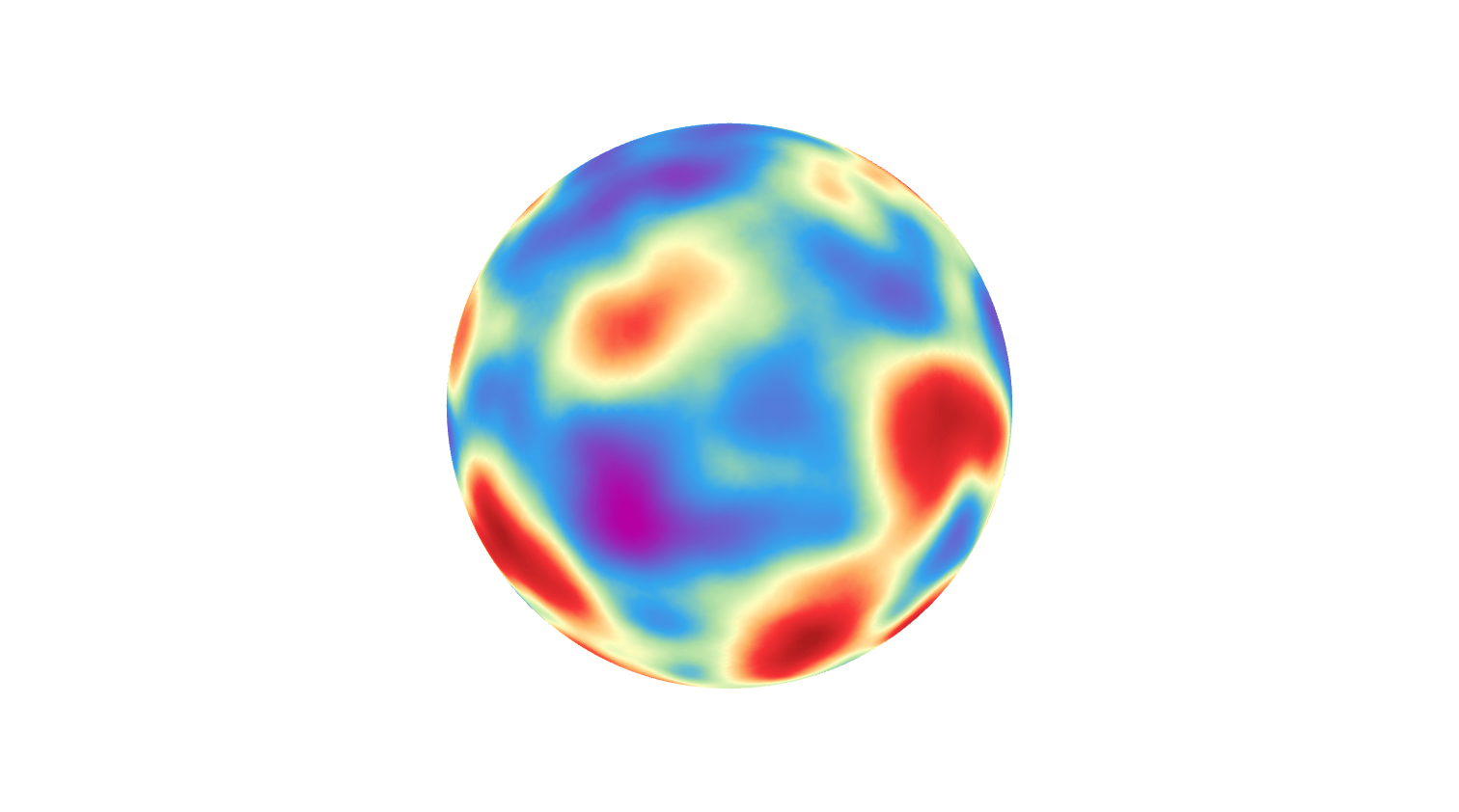
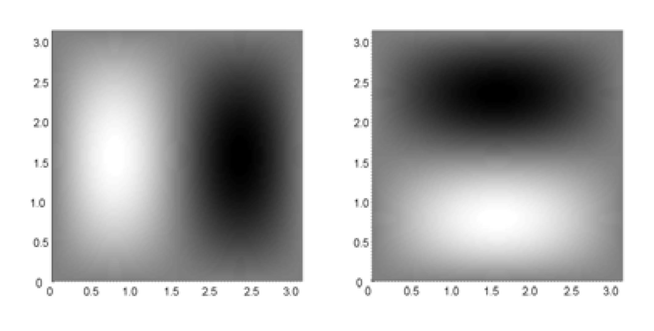
(Whittle-) Matérn random fields given by SPDE \((\kappa^2-\Delta_{\mathbb{S}^2})^\beta \mathcal Z = \mathcal{W}\)!
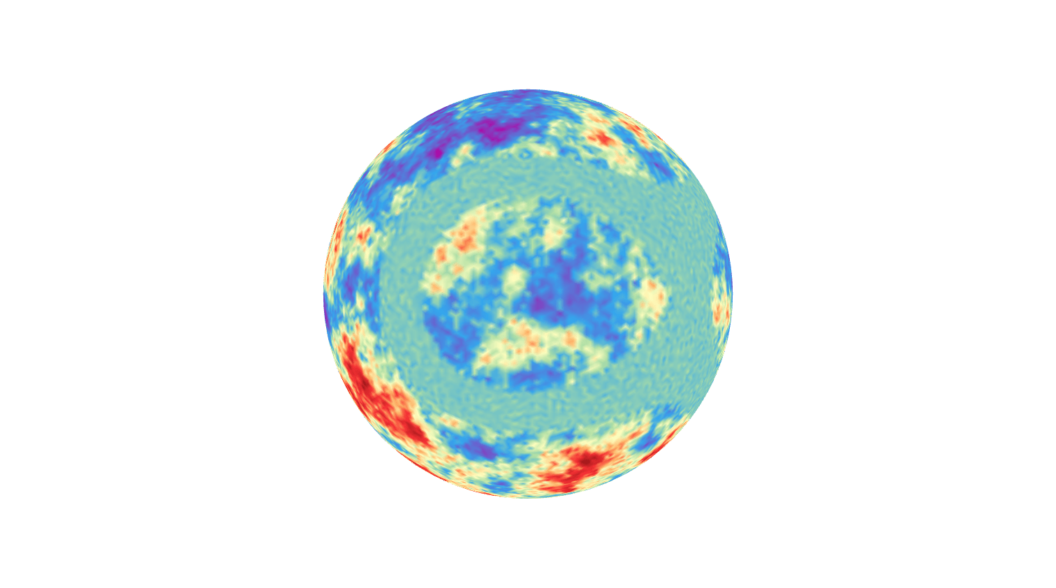
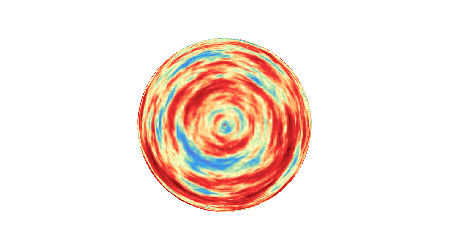
\(\rho_1\) small, \(\rho_2\) large: field is elongated tangentially along level sets of \(f\)
\(\rho_1\) large, \(\rho_2\) small: field is elongated orthogonally along level sets of \(f\)
Problem: \((\lambda_i,e_i)\) is not available!
Sampling \(\iff\) Evaluating \(\mathcal Z = \sum_{i=1}^\infty \gamma(\lambda_i) W_i e_i\)
Can \((\lambda_i,e_i)\) be approximated?
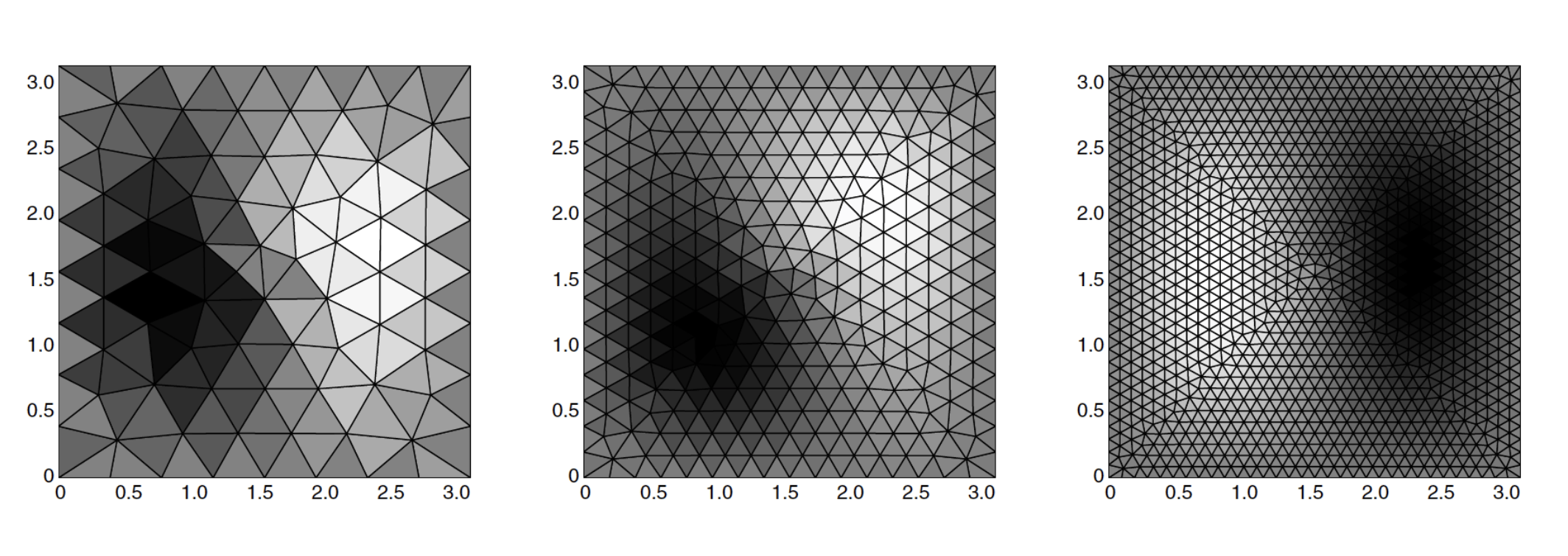
Maybe? Solving an SPDE, try with FEM!
On Euclidean spaces
Just triangulate the domain!
Put the pieces back together, get the original domain!
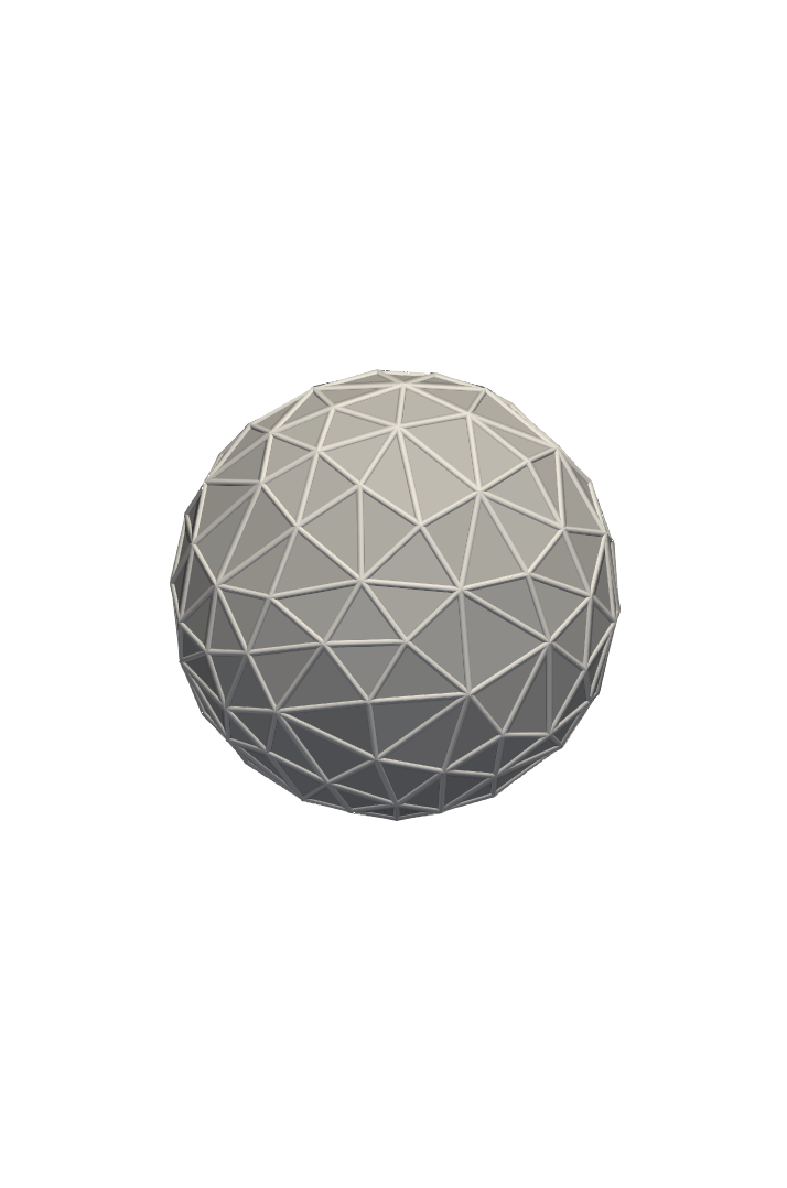
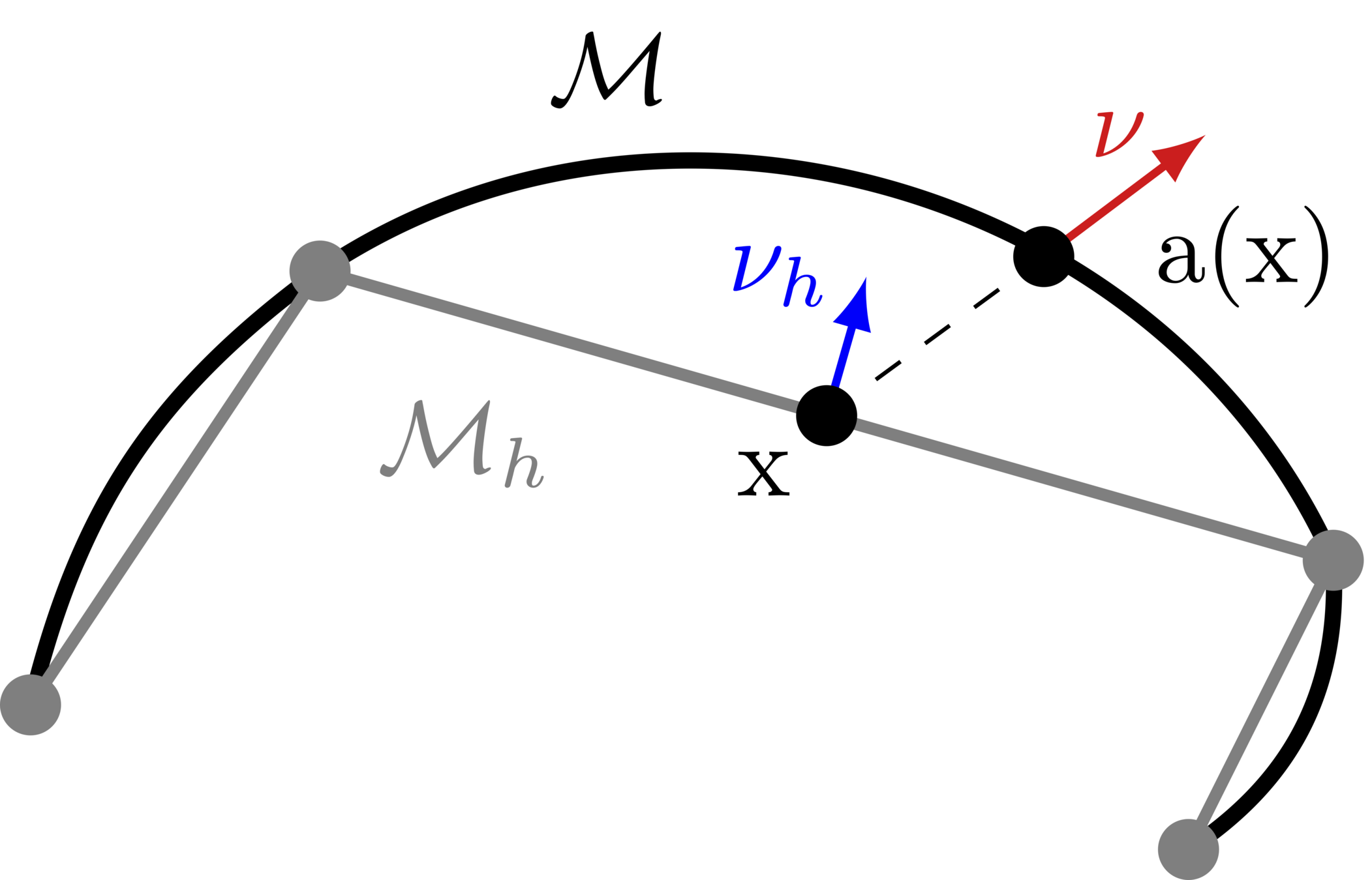
On manifolds!
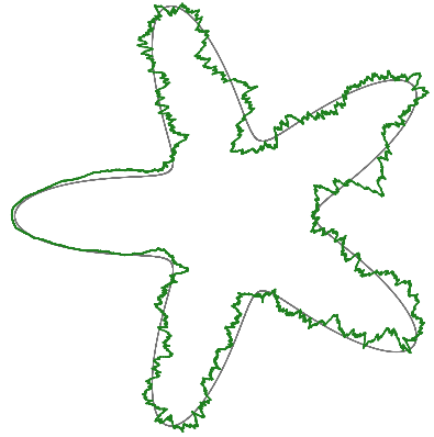
Step 1: Triangulate the domain
Issue: Approximate solutions live on \(\mathcal{M}_h\), not \(\mathcal{M}\)!
Put the pieces back together, don't get the same domain!
Step 2: FEM space \(S_h \subset H^1(\mathcal{M}_h)\) of p.w., continuous, linear functions
Step 3: Key tool in surface finite elements: the lift
Takeway: FEM error similar to flat case, up to a "geometry error" term
Discretization of operators
Original
Eigenpairs
Discrete 1
Eigenpairs
Discrete 2
Eigenpairs
Use eigenpairs \((\Lambda_{i,h},E_{i,h})\) of \(\mathsf{L}_h\)
First idea: Use these to approximate
In practice:
Works with known mesh, "unknown" manifold:
Find a mesh and you can simulate GRFs on it!
What about strong error?
\((Z_i)\) are Gaussian with covariance matrix determined by \(\gamma\) and FEM matrices
Chebyshev quadrature approximation of \(\gamma\)
First try:
Problem:
Generally: Approximating eigenfunctions are hard!
Eigenvalues are fine, however!
Generally: Approximating eigenfunctions are hard! Multiplicity!
From D. Boffi, Acta Num. (2010)
Various white noise approximations, various approximations of \(\mathcal Z\)
sd
sd
sd
??
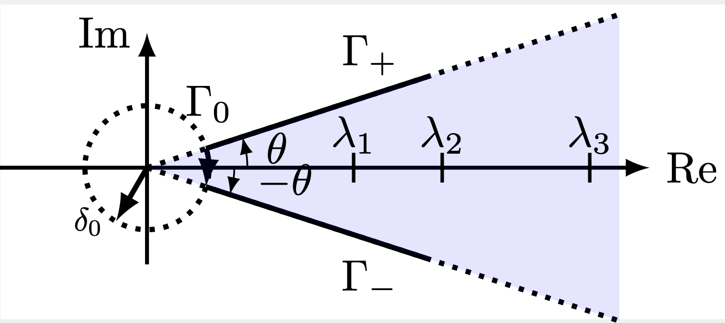
Important result: errors on the form
\(\|\gamma(\mathcal L)f -\gamma(\mathcal L_h) f\|_{L^2}\)
Brief note on proof:
Brief note on proof:
In the end:
By Erik Jansson


