


federica bianco PRO
astro | data science | data for good
Fall 2025 - UDel PHYS 461-66
dr. federica bianco
@fedhere
WRITTEN FINAL:
72 hours at home
Dec 11 8AM - Dec 14 8AM
WORK ALONE
USE AI AT YOUR OWN RISK
USE THE SLACK CHANNEL FOR QUESTIONS
DM ME IF YOUR QUESTION REQUIRES SHARING CODE OR SOLUTIONS
WRITTEN FINAL:
72 hours at home
Dec 11 8AM - Dec 14 8AM
WORK ALONE
USE AI AT YOUR OWN RISK
USE THE SLACK CHANNEL FOR QUESTIONS
DM ME IF YOUR QUESTION REQUIRES SHARING CODE OR SOLUTIONS
ORAL FINAL:
Schedule 30 minutes with me
in those 30 minutes I will ask you questions about things you did in your final
You shall demonstrate that :
- you understand what you did
- you made informed choices based on what you leanred in the class
- you can answer questions about data science topics (e.g. what other method could you have used? or why would a NN not be a good choice here?)
FINAL!!
Study Material:
conceptually
-> review slides, look at quiz questions you got wrong
Coding and models:
-> review old assignments and labs. Note that "solutions" to the HWs are posted int he HW folder on https://github.com/fedhere/DSPS_FBianco
Tasks you will need to complete in the final:
Tasks you will need to complete in the final:
Tasks you will need to complete in the final:
Tasks you will need to complete in the final:
Tasks you will need to complete in the final:
Tasks you will need to complete in the final:
Tasks you will need to complete in the final:
Tasks you will need to complete in the final:
Tasks you will need to complete in the final:
all ** tasks need justification explanation and interpretation!
and all plots need WHAT to count?
Tasks you will need to complete in the final:
all ** tasks need justification explanation and interpretation!
and all plots need captions that described the "what" the "how" and the "WOW"
ATTENTION! exploratory data analysis is critical!!!
tasks include:
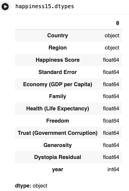
- look at datatypes
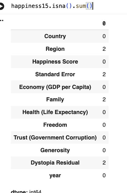
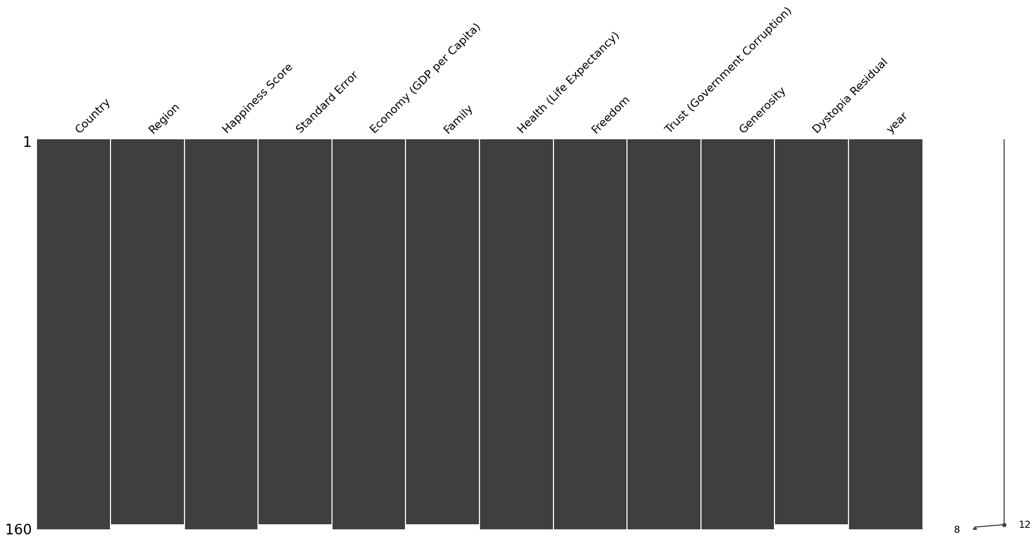
- ascertaining presence of NaN or missing values (e.g. -999) and devising and justifying a strategy to deal with them
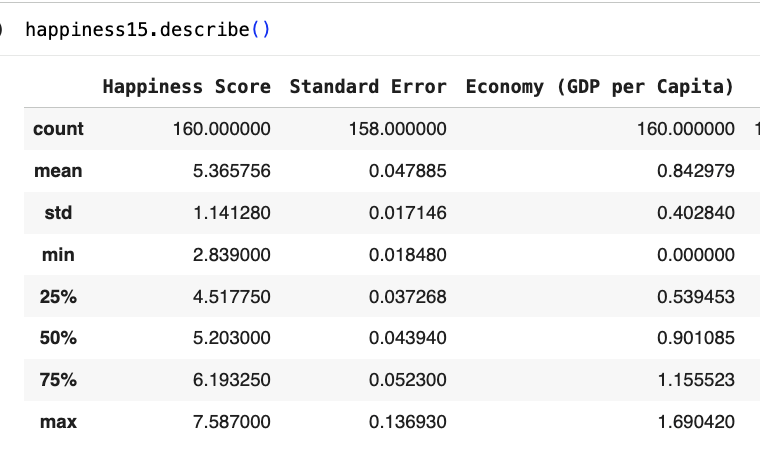
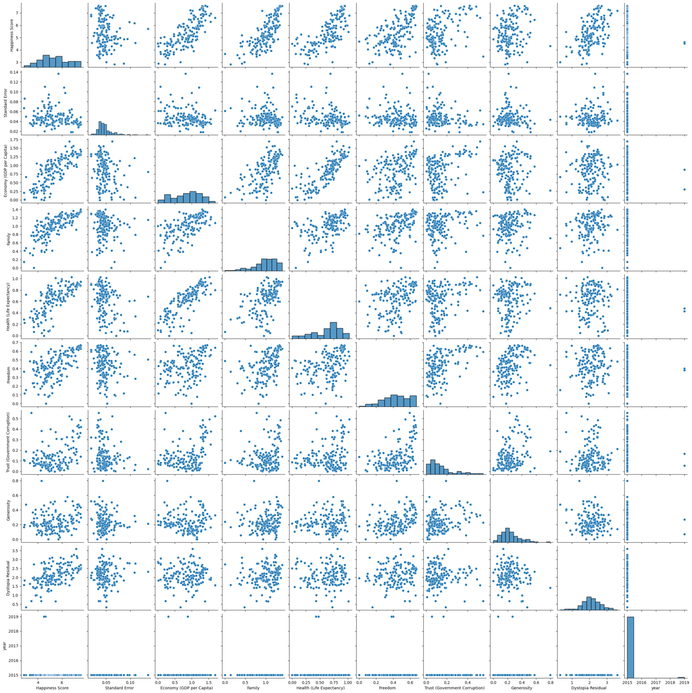
- ascertaining the distribution of imput features
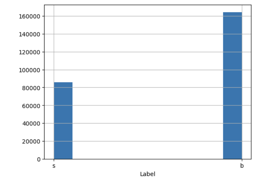
- ascertaining the distribution of target features! (e.g. howo many instances of each class, is the target value balanced??)
- ascertaining the correlation and covariance structure of the data!
ATTENTION! exploratory data analysis is critical!!!
tasks include:
- look at datatypes
- ascertaining presence of NaN or missing values (e.g. -999) and devising and justifying a strategy to deal with them
- ascertaining the distribution of imput features
- ascertaining the distribution of target features! (e.g. howo many instances of each class, is the target value balanced??)
- ascertaining the correlation and covariance structure of the data!
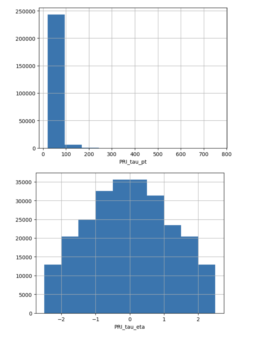
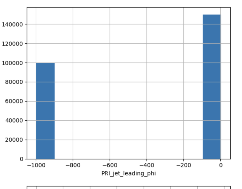
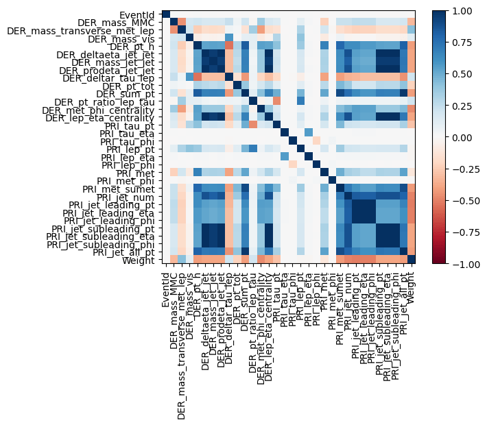
Higgs Boson
used -999 as missing value! ->
ATTENTION! exploratory data analysis is critical!!!
tasks include:
- look at datatypes
- ascertaining presence of NaN or missing values (e.g. -999) and devising and justifying a strategy to deal with them
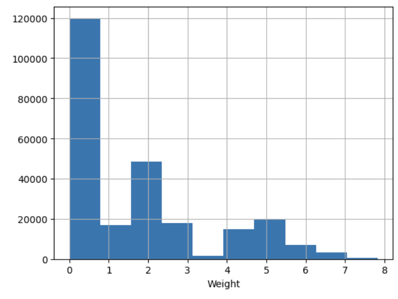
- ascertaining the distribution of imput features
- ascertaining the distribution of target features! (e.g. howo many instances of each class, is the target value balanced??)
- ascertaining the correlation and covariance structure of the data!
ATTENTION! exploratory data analysis is critical!!!
tasks include:
- look at datatypes
- ascertaining presence of NaN or missing values (e.g. -999) and devising and justifying a strategy to deal with them
- ascertaining the distribution of imput features
- ascertaining the distribution of target features! (e.g. howo many instances of each class, is the target value balanced??)
- ascertaining the correlation and covariance structure of the data!
And for all of this:
WHAT DOES IT MEAN?
HOW DOES IT GUIDE YOUR DATA PREP CHOICES?
HOW DO YOU USE IT TO CHOOSE YOUR MODEL?
HOW DOES IT INFLUENCE YOUR RESULT?
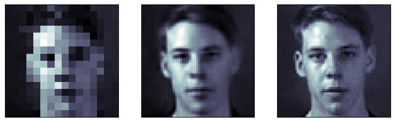
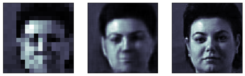
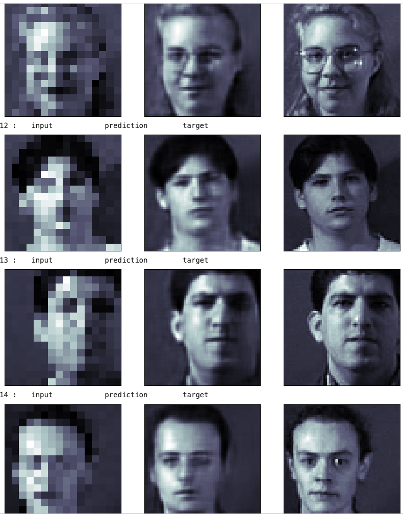
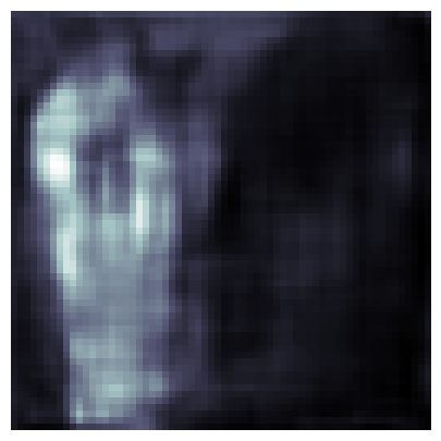
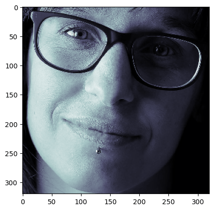
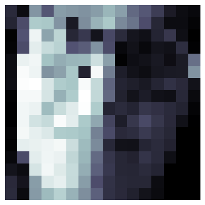
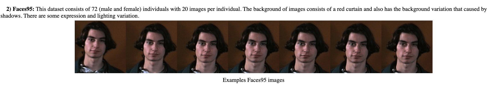
White Males: 43
White Female: 6
Non-White Males: 12
Non-White Female: 1
Faces95 - Computer Vision Science Research Projects, Dr Libor Spacek.
The dataset was BIASED -> the model was BIASED
The model was not transferable
1
The central dogma of molecular biology is: Structure Determines Function.
Enzymes: The precise 3D shape creates an "active site" where specific chemical reactions are catalyzed. The wrong shape means no reaction.
Antibodies: Their Y-shaped structure allows them to recognize and bind to foreign invaders like viruses and bacteria.
Structural Proteins (e.g., Collagen, Keratin): Their folded shapes provide strength and support to tissues like skin, hair, and bones.
Transport Proteins (e.g., Hemoglobin): Their shape allows them to pick up and release oxygen in the blood.
Proteins are:
Polymers of amino acids. The sequence of amino acids is recorded in your DNA
The amino acid sequence determines the folded structure of the protein
The folded structure has evolved to support the function of the protein
The information needed for folding is encoded in the protein's amino acid sequence, which itself is encoded in DNA.
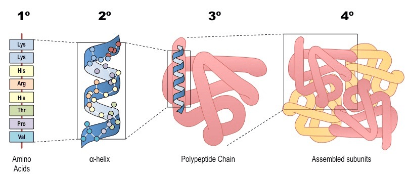
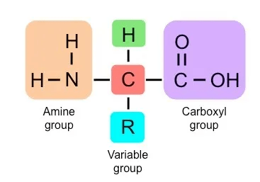
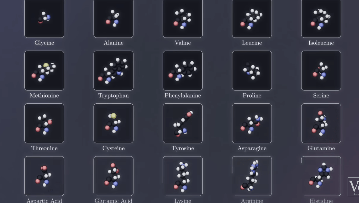
1 - Amino Acid Sequence (Primary Structure): The arrangement of amino acids in a protein. The DNA code is translated into a linear chain of amino acids. Proteins can be made from 20 different amino acids, and the structure and function of each protein are determined by the kinds of amino acids used to make it and how they are arranged.
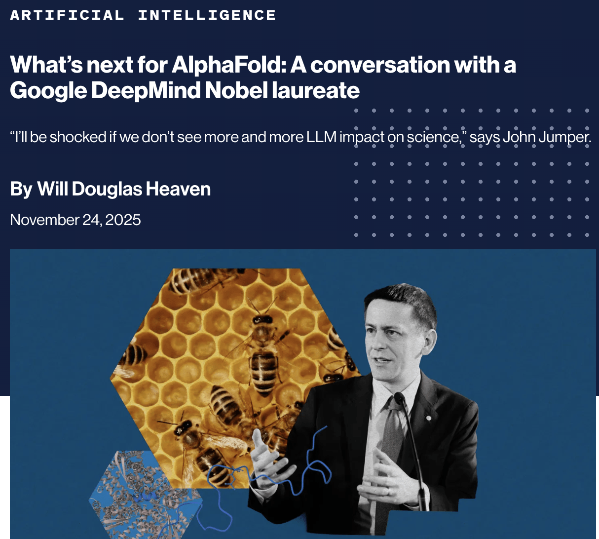
The wild, wonderful world of proteins
https://youtu.be/_GPDsQnnvrA?t=48
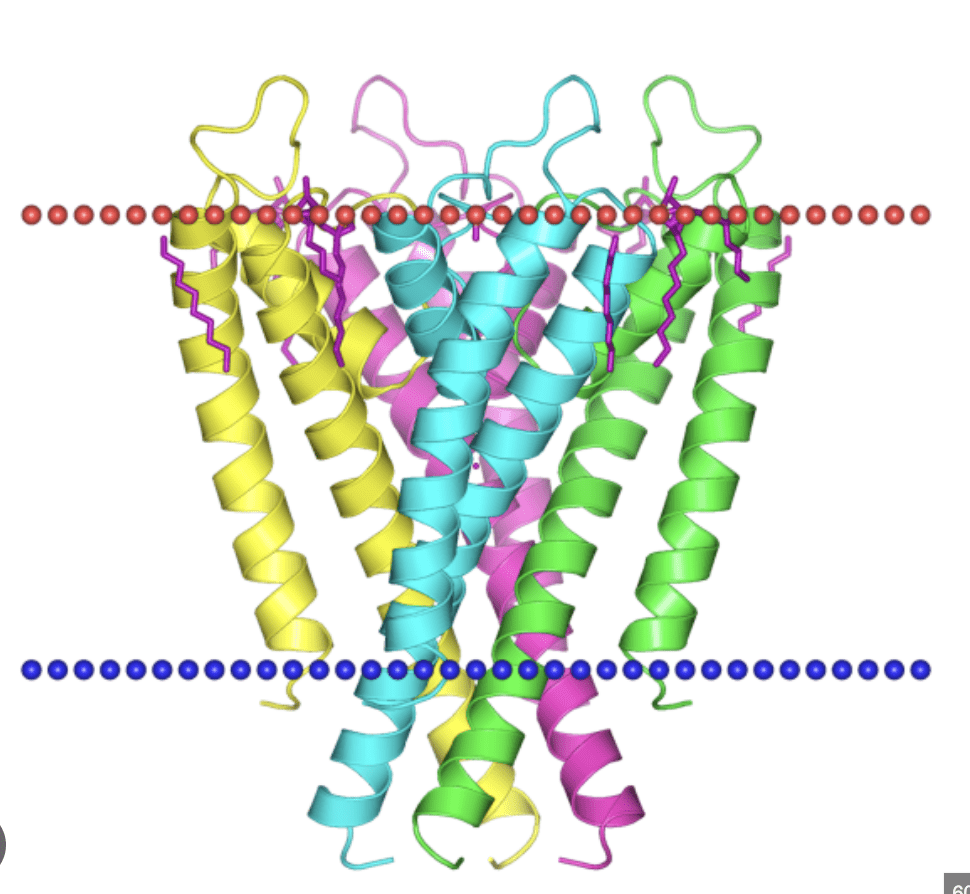
proteins are channels for ions...
...transporters of O2 and other molecules...
...transducers of chemical energy
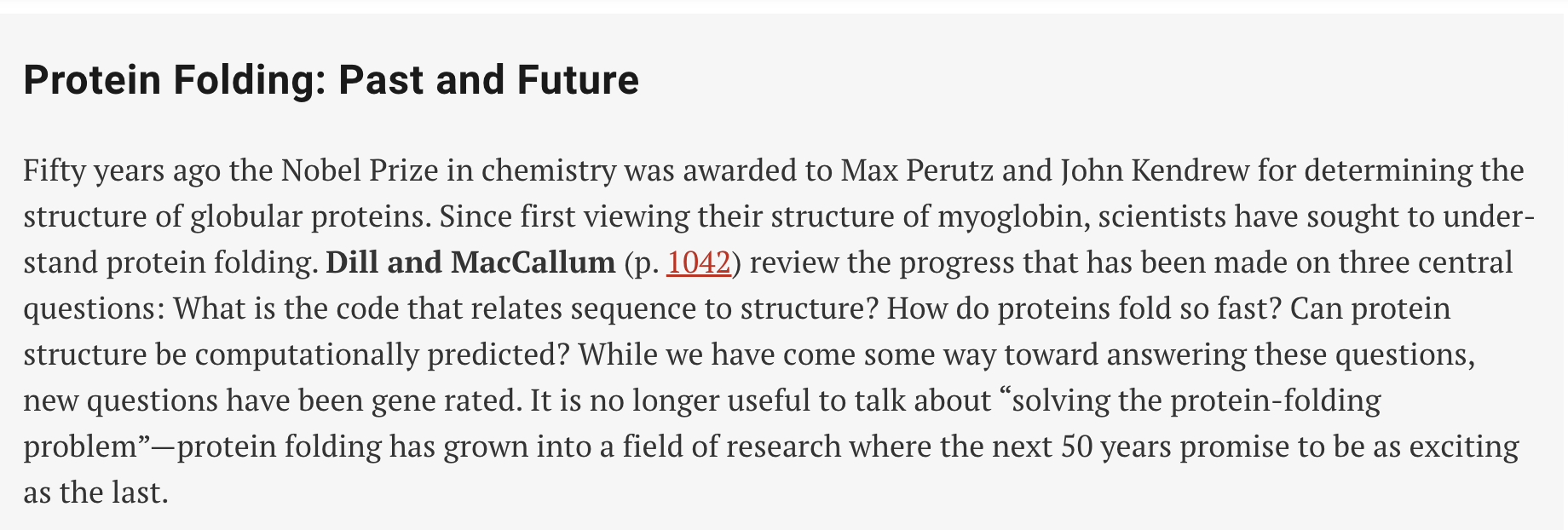
Why does protein structure matter?
Because structure determines function. And function is biology!
Where do we get a protein structure?
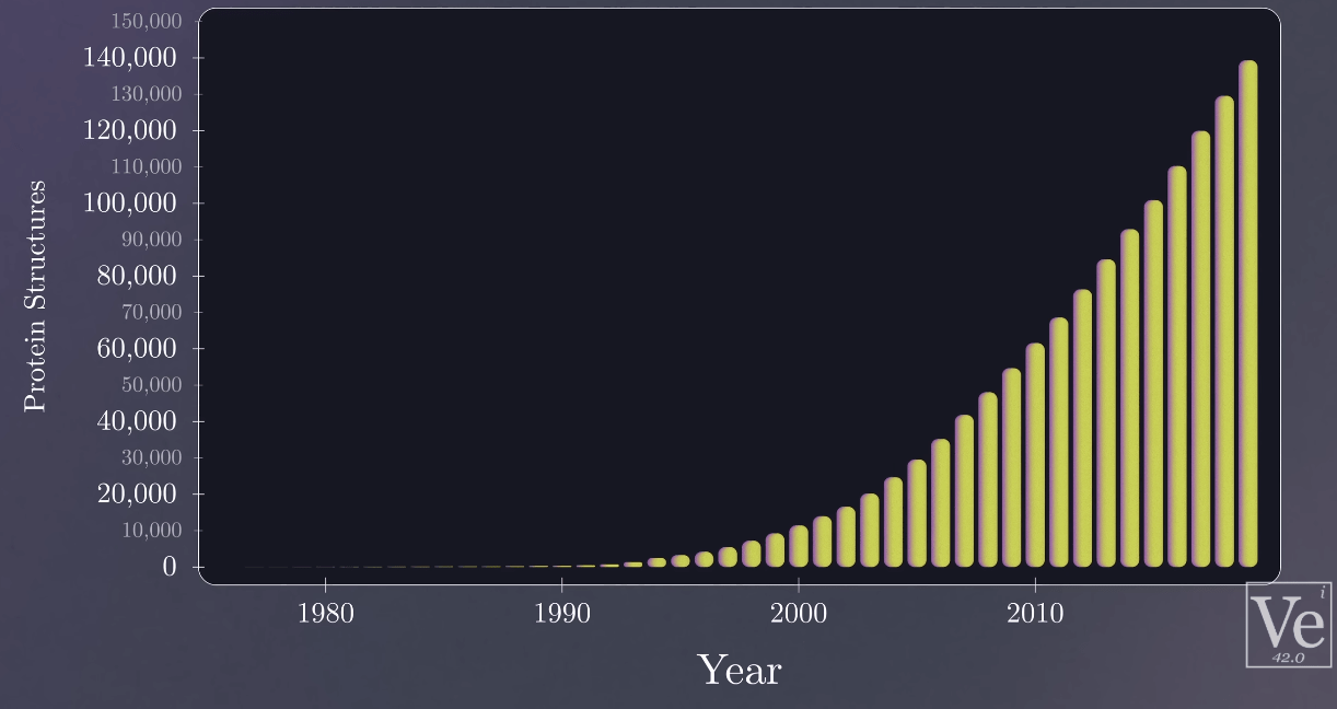
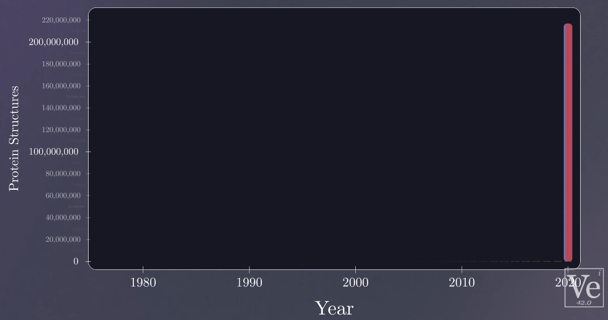
There are 246,045 of them determined experimentally and deposited into the "PDB"
Experiments to "solve" protein structures are: hard, time consuming, $$$$ (and not strictly experimental)
Wouldn't it be great if we had a magic box where we could input the sequence and get a prediction for the structure??
How it works: It uses a deep learning network trained on the thousands of known protein structures in the Protein Data Bank (PDB). It looks for evolutionary patterns and physical constraints to predict the 3D coordinates of every atom.
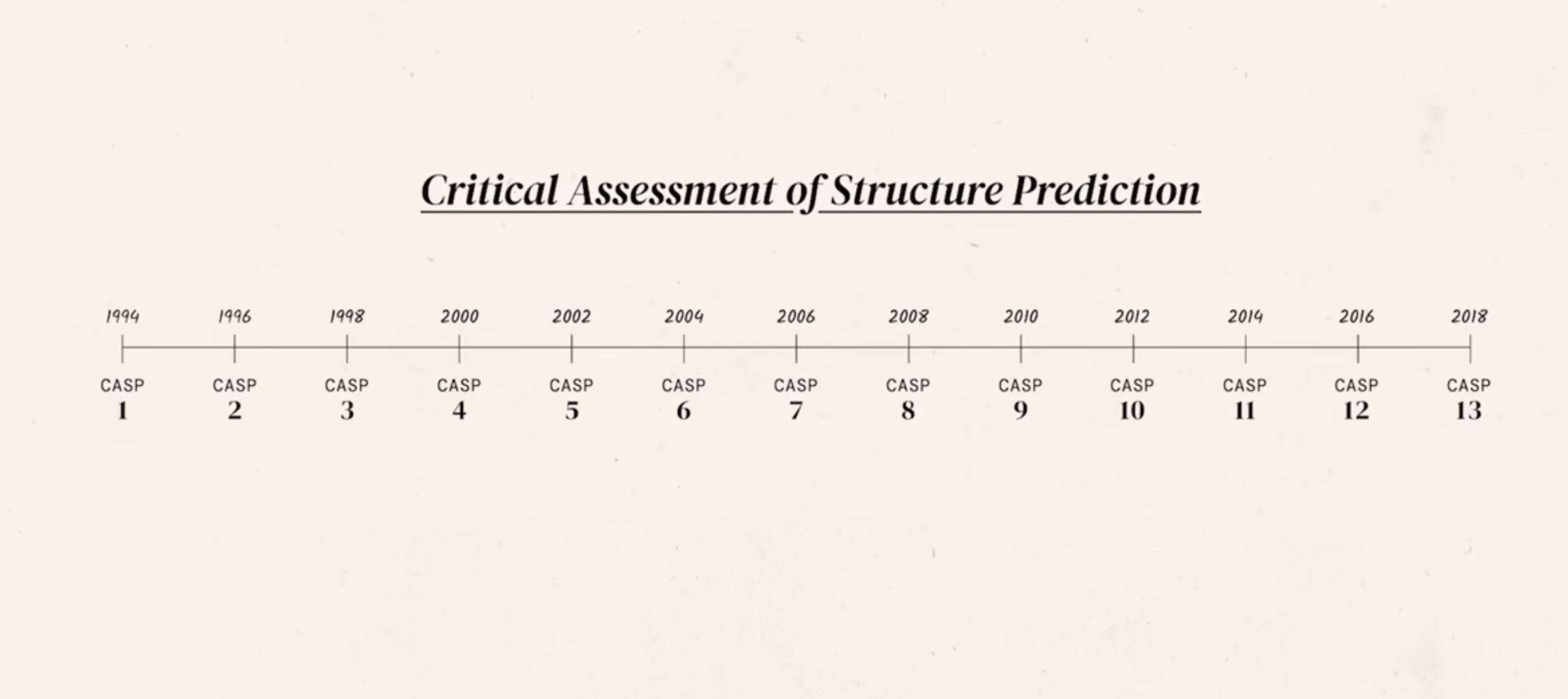
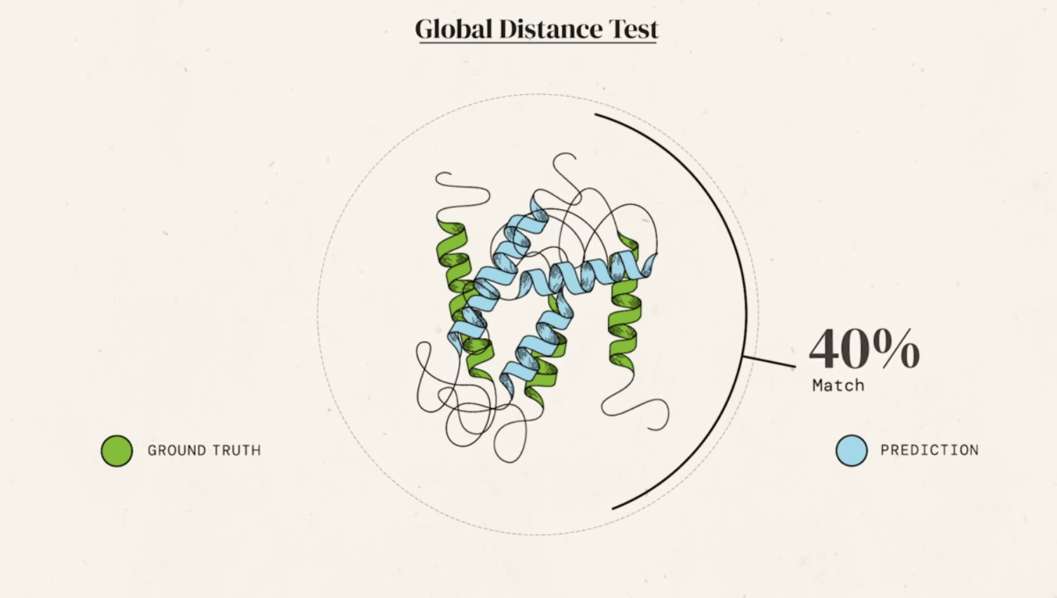
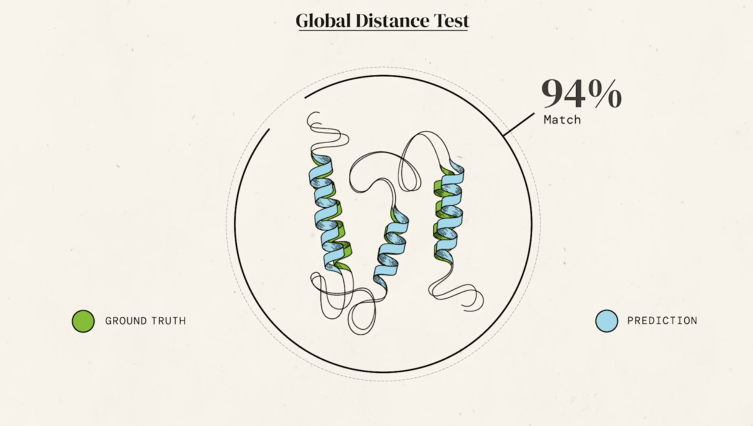
send out groups of 100 proteins and ask researchers to predict folding
How it works: It uses a deep learning network trained on the thousands of known protein structures in the Protein Data Bank (PDB). It looks for evolutionary patterns and physical constraints to predict the 3D coordinates of every atom.
How it works: It uses a deep learning network trained on the thousands of known protein structures in the Protein Data Bank (PDB). It looks for evolutionary patterns and physical constraints to predict the 3D coordinates of every atom.
How it works: It uses a deep learning network trained on the thousands of known protein structures in the Protein Data Bank (PDB). It looks for evolutionary patterns and physical constraints to predict the 3D coordinates of every atom.
How it works: It uses a deep learning network trained on the thousands of known protein structures in the Protein Data Bank (PDB). It looks for evolutionary patterns and physical constraints to predict the 3D coordinates of every atom.
How it works: It uses a deep learning network trained on the thousands of known protein structures in the Protein Data Bank (PDB). It looks for evolutionary patterns and physical constraints to predict the 3D coordinates of every atom.
AlphaFOLD2
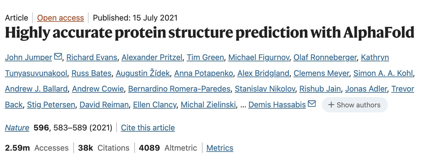
AF3 (~9,000 citations)
AF2 (~40,000 citations)
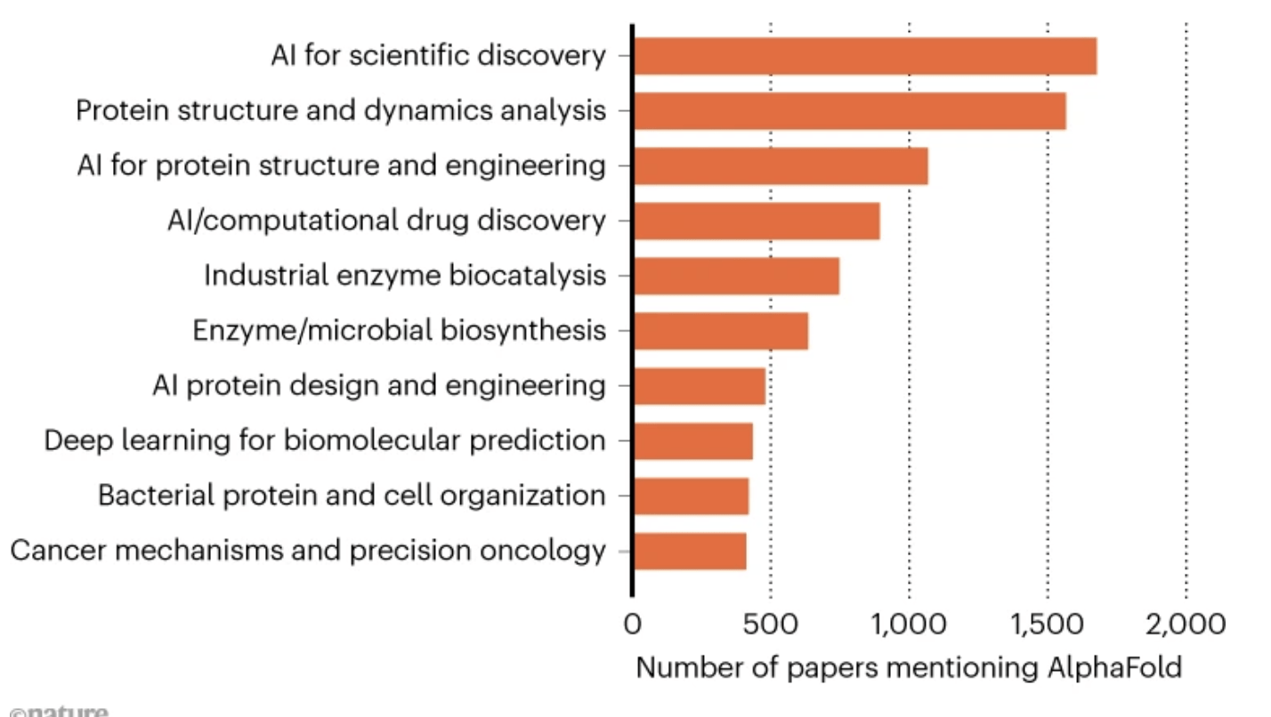
New Science enabled by alphafold
Any question that needs a structure to make progress! (And if that was your PhD thesis...oopsie!)
Searching a database by of proteins by structure instead of sequence
https://doi.org/10.1038/d41586-025-03886-9
Predicting the effects of "missense" mutations
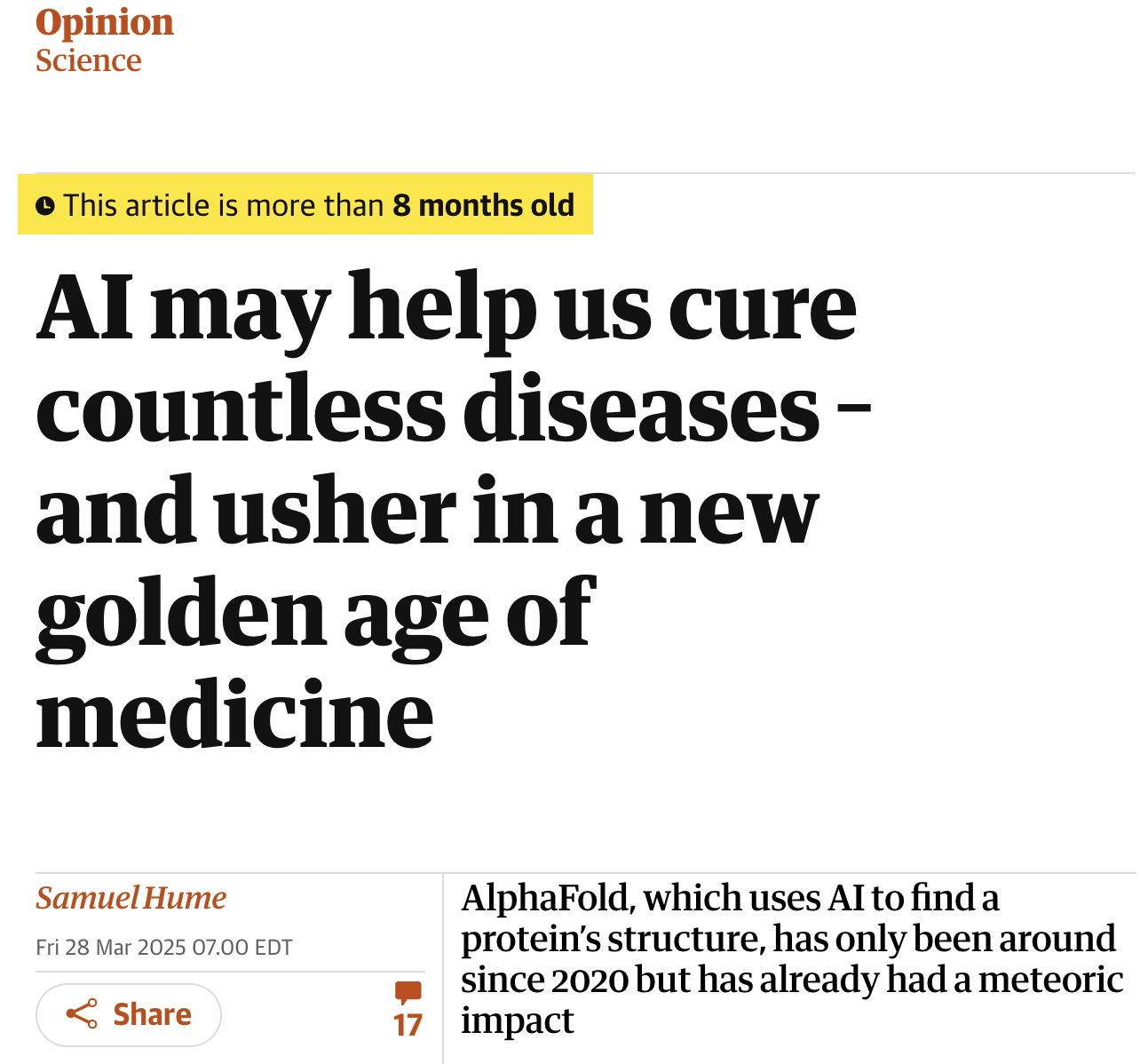
But maybe also slow your roll, bruh
What can AF not do? Or maybe — what has been over promised?
The information needed for folding is encoded in the protein's amino acid sequence, which itself is encoded in DNA.
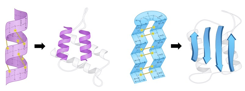
2 Local Folding (Secondary Structure): Sections of the chain spontaneously form local, stable patterns held together by hydrogen bonds. The most common are:
α-helices: A coiled, spring-like structure.
β-sheets: Pleated strands that line up side-by-side.
It is the way a polypeptide folds in a repeating arrangement.
This folding is a result of H bonding between the amine and carboxyl groups of non-adjacent amino acids
The information needed for folding is encoded in the protein's amino acid sequence, which itself is encoded in DNA.
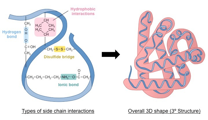
3 Global Folding (Tertiary Structure): The entire chain folds further into a unique, compact 3D shape.
The information needed for folding is encoded in the protein's amino acid sequence, which itself is encoded in DNA.
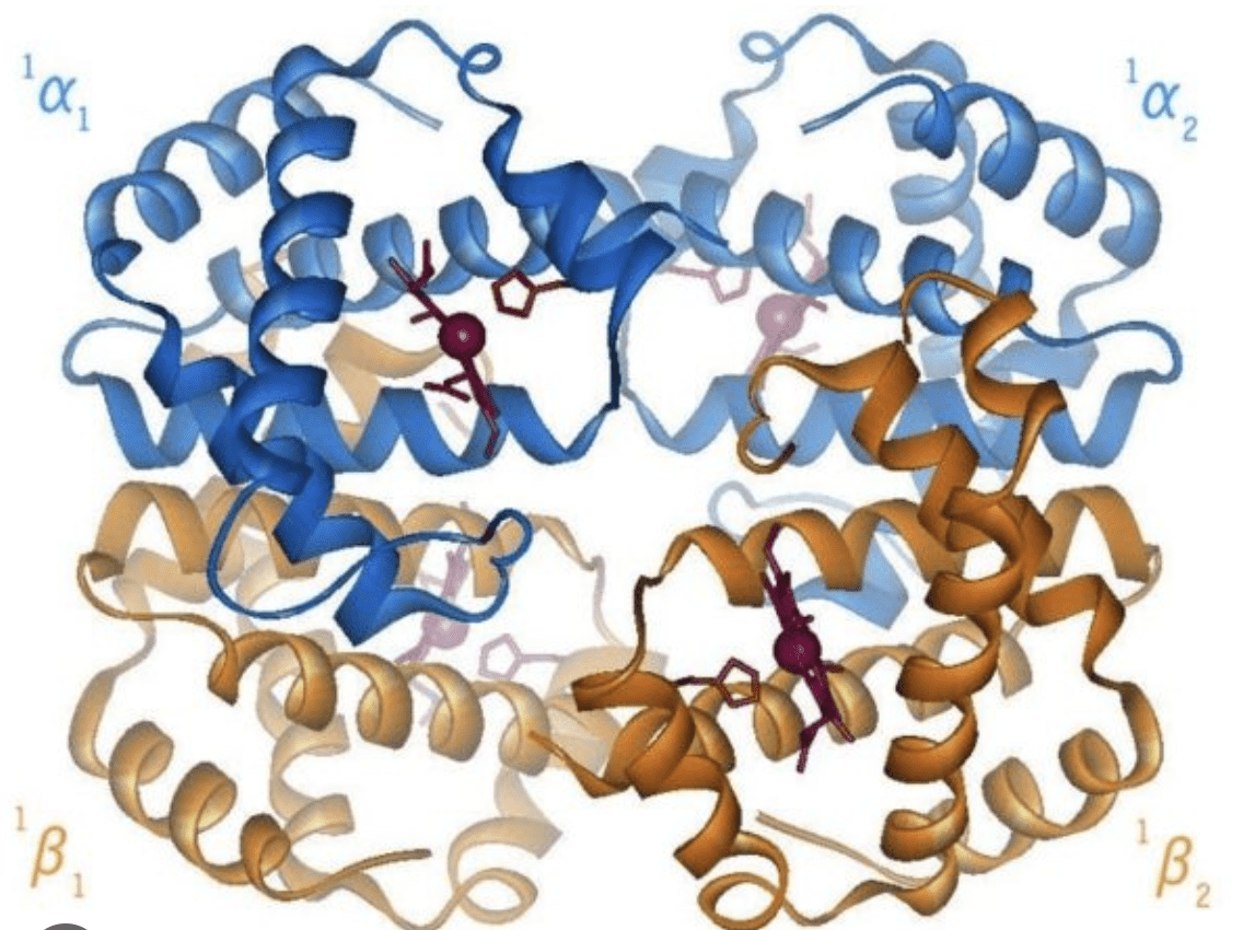
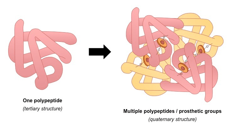
4 Complex Assembly (Quaternary Structure): Some proteins are made of multiple folded polypeptide chains (subunits) that assemble together to form the final, functional protein (e.g., hemoglobin).
Drug Design (Structure-Based Drug Design): Most drugs work by binding to a specific protein to either activate or block its function: design drugs to perfectly fit into a protein active site.
Example: Predicting the structure of the SARS-CoV-2 spike protein was crucial for rapidly developing vaccines and therapeutic antibodies
Understanding Genetic Diseases
Fighting "Misfolding" Diseases: Alzheimer's and Parkinson's,
Motivation
Anfinsen’s dogma
In standard physiological environment, a protein’s structure is determined by the sequence of amino acids that make it up (1972 Nobel Prize in Chemistry).
If so we should be able to reliably predict a protein’s structure from its sequence.
Levinthal’s paradox
In the 1960s, Cyrus Levinthal showed that finding the native folded state of a protein by a random search among all possible configurations can take a time comparable with the lifetime of the Universe.
35 aminoacids ->1e33 ways to fold
A small and physically reasonable energy bias against locally unfavorable configurations, of the order of a few kT, can reduce Levinthal's time to a biologically significant size.
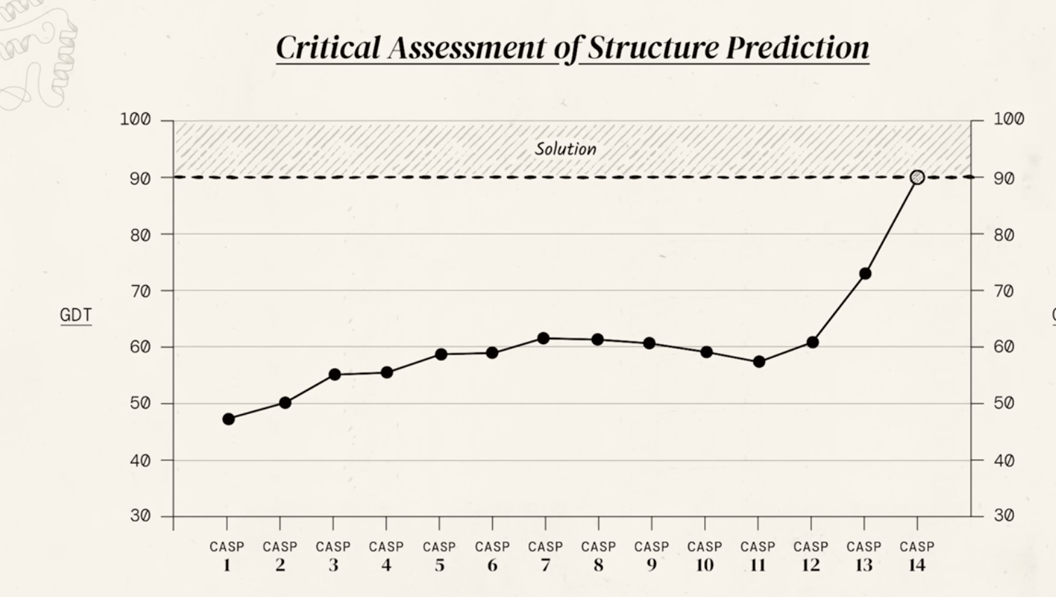
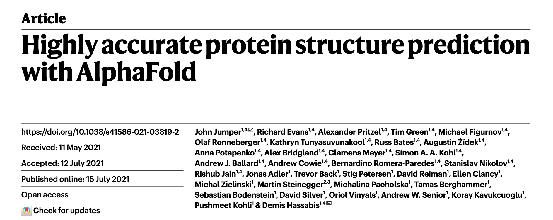
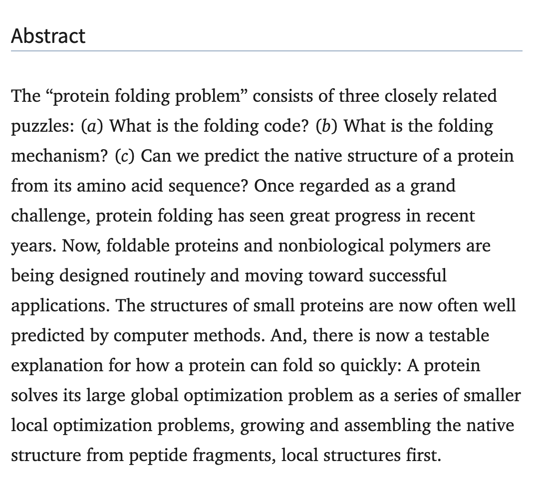
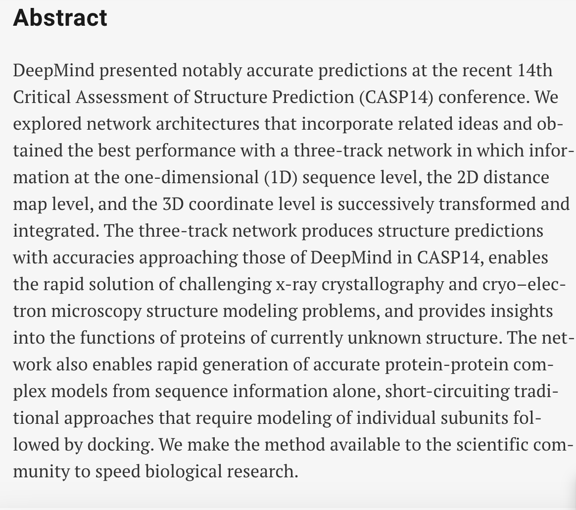
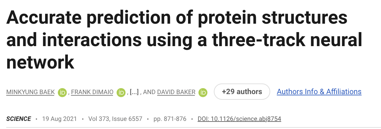
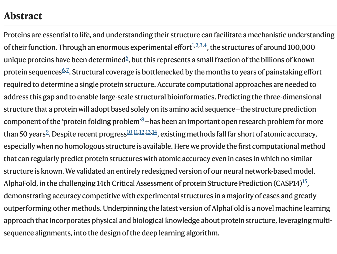
For decades, predicting a protein's 3D structure from its amino acid sequence alone (the "protein folding problem") was one of the grand challenges in biology. This was revolutionized in 2020 by DeepMind's AlphaFold, an artificial intelligence system.
1600+ citations
2100+ citations
2
In the 1960s Cyrus Levinthal shiwed that there is a large number of possible conformation that a protein could theoretically adopt and if a protein were just to try them all it would take a time comparable to the life of the Universe (~10 Gyears)
ok, some are obviously better than others, so you dont have to explore them ALL
140,000 protein structures found by 2014
AlphaFold greatly improves the accuracy of structure prediction by incorporating novel neural network architectures and training procedures based on the evolutionary, physical and geometric constraints of protein structures.
new equivariant attention architecture, use of intermediate losses to achieve iterative refinement of predictions, masked MSA loss to jointly train with the structure, learning from unlabelled protein sequences using self-distillation and self-estimates of accuracy.
In particular, we demonstrate a new architecture to jointly embed multiple sequence alignments (MSAs) and pairwise features, a new output representation and associated loss that enable accurate end-to-end structure prediction,
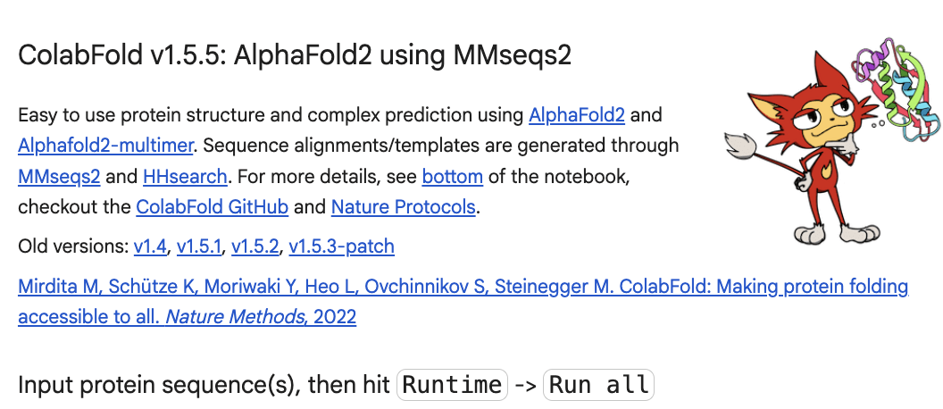
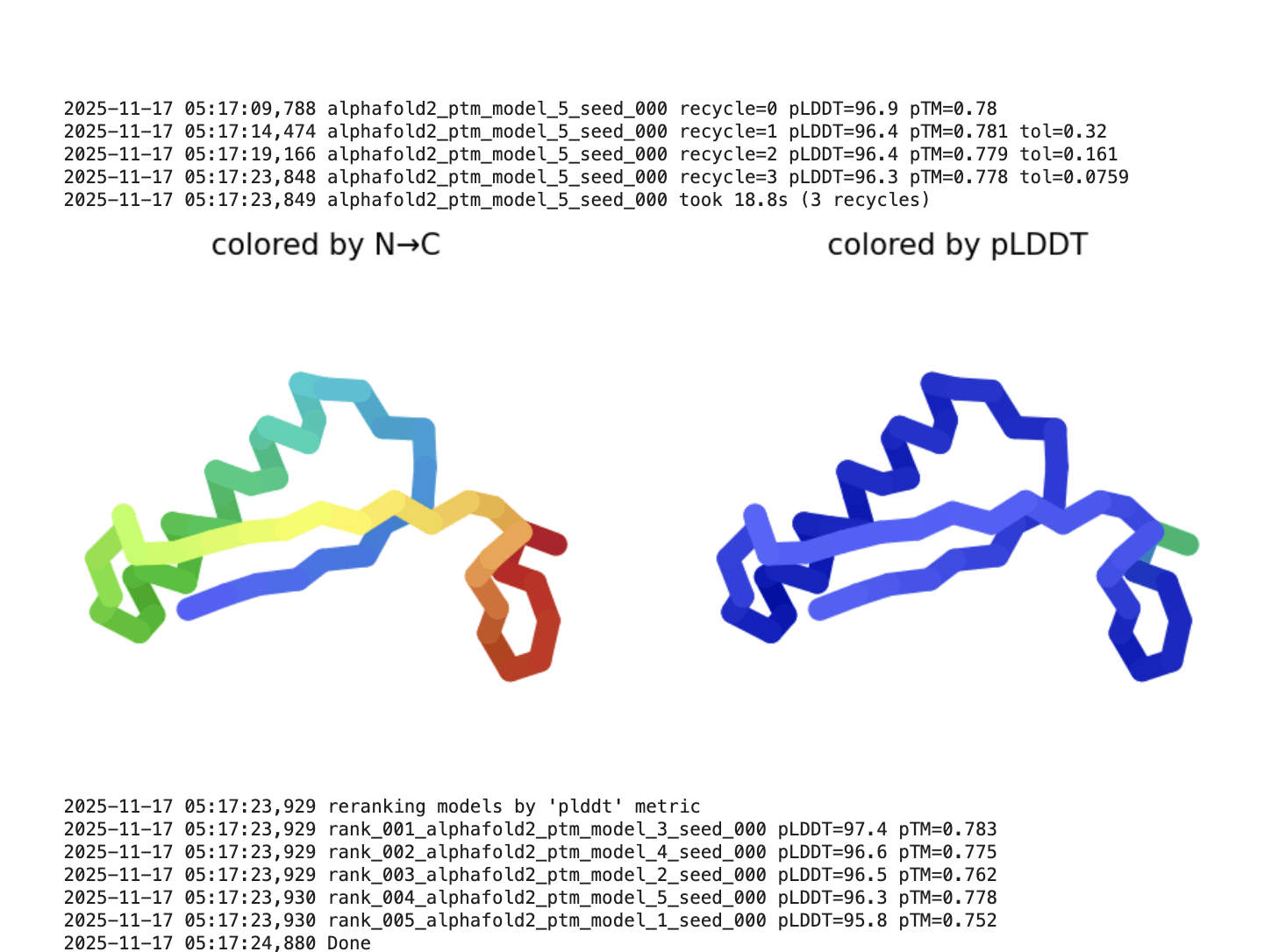
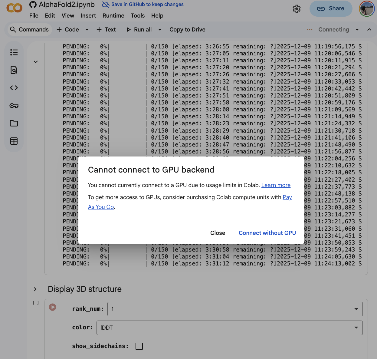
https://colab.research.google.com/github/sokrypton/ColabFold/blob/main/AlphaFold2.ipynb
https://colab.research.google.com/github/sokrypton/ColabFold/blob/main/AlphaFold2.ipynb
Innovative Input and Ouptut
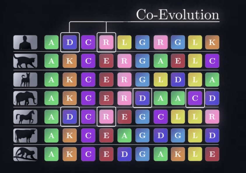
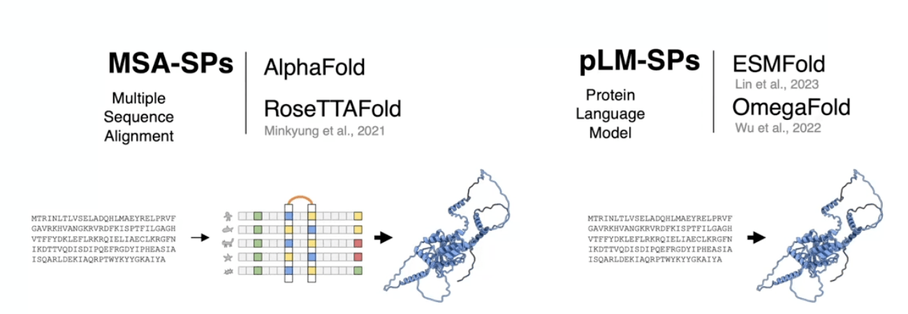
Multi Sequence Allignment
Innovative Input and Ouptut
Multi Sequence Allignment
pairs preserved in multiple spicies: coevolution
Innovative Input and Ouptut
Multi Sequence Allignment
changes that occurr in pairs
pairs preserved in multiple spicies: coevolution
Innovative Input and Ouptut
Multi Sequence Allignment
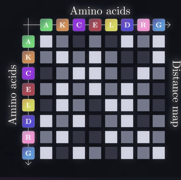
Distance Matrix
changes that occurr in pairs
pairs preserved in multiple spicies: coevolution
G-A close together in the final structure
Innovative Input and Ouptut
Multi Sequence Allignment
Distance Matrix
changes that occurr in pairs
pairs preserved in multiple spicies: coevolution
G-A close together in the final structure
D-E are distant in the final structure
Innovative Input and Ouptut
Multi Sequence Allignment
Distance Matrix + Torsion Angles
changes that occurr in pairs
pairs preserved in multiple spicies: coevolution
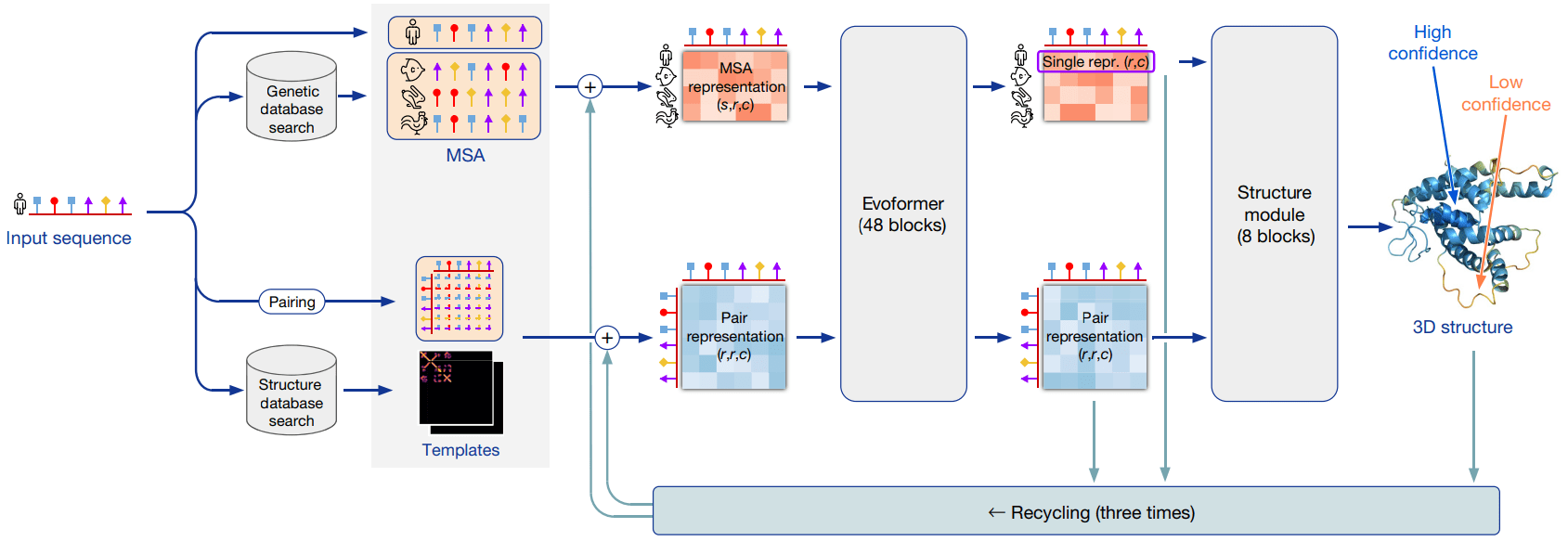
Instead of directly predicting 3D coordinates, AlphaFold's neural network was trained to predict two intermediate representations:
Distogram: A matrix of pairwise distances between every amino acid residue in the protein. This defines the protein's fold topology.
Torsion Angles: The internal rotation angles of the protein backbone (phi and psi angles).
Torsion Angles
CASP gives 1 sequence
additional input:
examples of similar
protein sequences
in their folded form
How it works: It uses a deep learning network trained on the thousands of known protein structures in the Protein Data Bank (PDB). It looks for evolutionary patterns and physical constraints to predict the 3D coordinates of every atom.
AlphaFold ->
2018
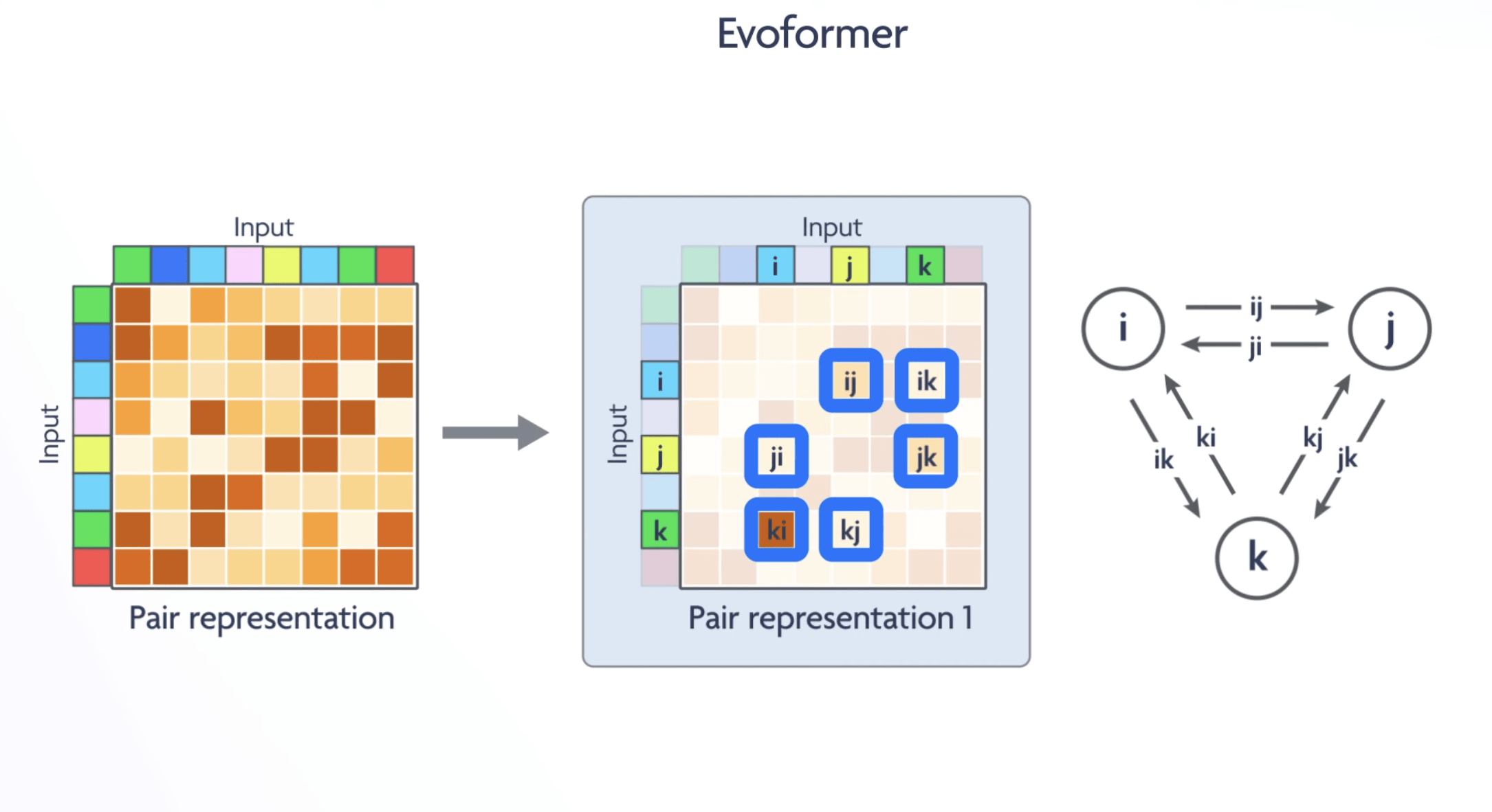
new architecture to jointly embed multiple sequence alignments (MSAs) and pairwise features
A 3D tensor of shape
(N_seq, N_res, c_m).
c_m =256 in AlphaFold2
CASP gives 1 sequence
Multiple Sequence Alignment
CASP gives 1 sequence
templates of folded proteins
A 3D tensor of shape
(N_res, N_res, c_z)
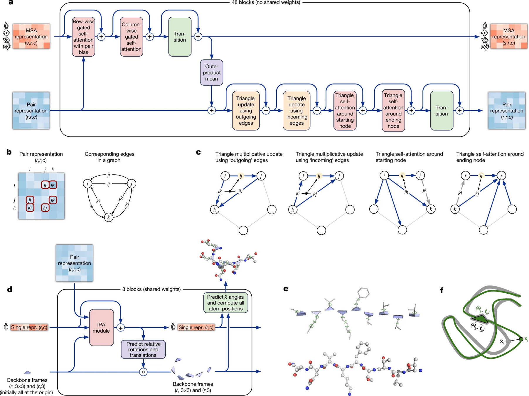
We show evidence in ‘Interpreting the neural network’ that a concrete structural hypothesis arises early within the Evoformer blocks and is continuously refined. The key innovations in the Evoformer block are new mechanisms to exchange information within the MSA and pair representations that enable direct reasoning about the spatial and evolutionary relationships.
Evoformer
Evoformer
Evoformer
Structure module
structure module that introduces an explicit 3D structure in the form of a rotation and translation for each residue of the protein (global rigid body frames).
Rotational - Translational - Physico-chemical constraints (think of a PINN!!)
Structure module
structure module that introduces an explicit 3D structure in the form of a rotation and translation for each residue of the protein (global rigid body frames).
Rotational - Translational - Physico-chemical constraints (think of a PINN!!)
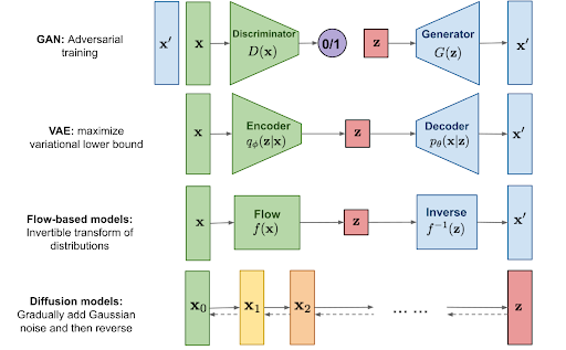
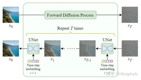
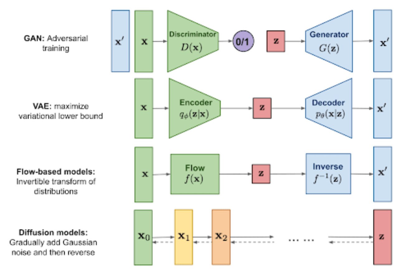
AlphaFold3: diffusion NN
new equivariant attention architecture, use of intermediate losses to achieve iterative refinement of predictions, masked MSA loss to jointly train with the structure, learning from unlabelled protein sequences using self-distillation and self-estimates of accuracy.
In particular, we demonstrate a new architecture to jointly embed multiple sequence alignments (MSAs) and pairwise features, a new output representation and associated loss that enable accurate end-to-end structure prediction,
How it works: It uses a deep learning network trained on the thousands of known protein structures in the Protein Data Bank (PDB). It looks for evolutionary patterns and physical constraints to predict the 3D coordinates of every atom.
AlphaFOLD2 ->
2020
2018
In the 1960s Cyrus Levinthal shiwed that there is a large number of possible conformation that a protein could theoretically adopt and if a protein were just to try them all it would take a time comparable to the life of the Universe (~10 Gyears)
ok, some are obviously better than others, so you dont have to explore them ALL
140,000 protein structures found by 2014
200,000,000 protein structures found by AlphaFols2/3
Compared to Large Language Models (LLMs): AlphaFold 2's cost is substantial but still an order of magnitude less than the largest LLMs. Training GPT-3 (2020) was estimated at $4-5 million, and more recent models like GPT-4 or Gemini Ultra likely cost over $100 million.
DeepMind (Google's AI division) has not released an official, precise figure. However, the consensus among experts is that the training cost for AlphaFold 2 was between $1 to $2 million USD in direct computational (cloud computing) expenses.
Fine Tuning Foundation Models
3
models trained extensively on large amounts of data to solve generic problems - typically selfsupervised (i.e. trained as generative AI to reproduce input data, dsps_12)
Foundational AI models
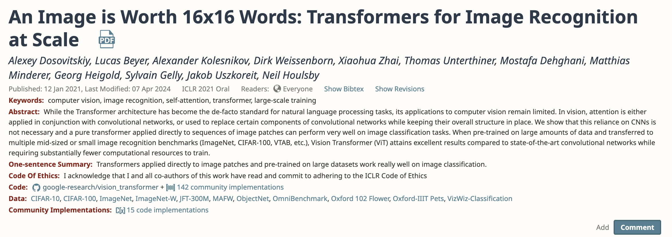
We use the ILSVRC-2012 ImageNet dataset with 1k classes
and 1.3M images, its superset ImageNet-21k with
21k classes and 14M images and JFT with 18k classes and
303M high-resolution images.
Typically, we pre-train ViT on large datasets, and fine-tune to (smaller) downstream tasks.
For this, we remove the pre-trained prediction head and attach a zero-initialized D × K feedforward
layer, where K is the number of downstream classes
models trained extensively on large amounts of data to solve generic problems - typically selfsupervised (i.e. trained as generative AI to reproduce input data)
Foundational AI models
We use the ILSVRC-2012 ImageNet dataset with 1k classes
and 1.3M images, its superset ImageNet-21k with
21k classes and 14M images and JFT with 18k classes and
303M high-resolution images.
Typically, we pre-train ViT on large datasets, and fine-tune to (smaller) downstream tasks.
For this, we remove the pre-trained prediction head and attach a zero-initialized D × K feedforward
layer, where K is the number of downstream classes
3 class classification problem
models trained extensively on large amounts of data to solve generic problems - typically selfsupervised (i.e. trained as generative AI to reproduce input data)
Foundational AI models
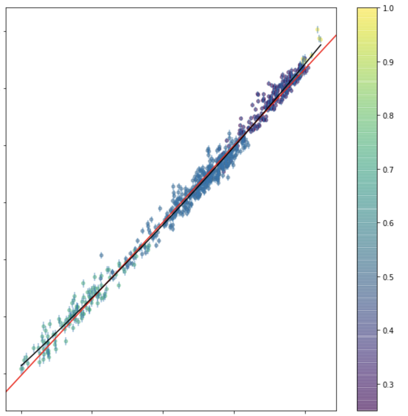
regression problem
We use the ILSVRC-2012 ImageNet dataset with 1k classes
and 1.3M images, its superset ImageNet-21k with
21k classes and 14M images and JFT with 18k classes and
303M high-resolution images.
Typically, we pre-train ViT on large datasets, and fine-tune to (smaller) downstream tasks.
For this, we remove the pre-trained prediction head and attach a zero-initialized D × K feedforward
layer, where K is the number of downstream classes
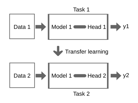
can you use it for another task?
you have a model which was trained on some data
DOMAIN ADAPTATION: learning a model from a source data distribution and applying that model on a target data with a different distribution: the features are the same but have different distributions
e.g. Learn an energy model in one city (using building size, usage, occupancy) then apply it to a different city
?
does the model generalize to answer question on the new dataset with accuracy?
YES
NO
No need for additional learning: the model is transferable!
Fine Tune your model on the new data
you have a model which was trained on some data
What problems does it solve?
Small labelled dataset for supervised learning: use a model trained on a larger related dataset (and possibly fine tune with small amount of labels)
Limited computational resources because more are not available or to limit environmental impact of AI, as low level learning can be reused
knowledge learned from a task is re-used in order to boost performance on a related task.
you have a model which was trained on some data
Industry models like Chat-GPT or SAM are trained on huge amount of data we scientists could not afford to get!
What problems does it solve?
Small labelled dataset for supervised learning: use a model trained on a larger related dataset (and possibly fine tune with small amount of labels)
Limited computational resources because more are not available or to limit environmental impact of AI, as low level learning can be reused
knowledge learned from a task is re-used in order to boost performance on a related task.
you have a model which was trained on some data
And large companies like Open-AI, Facebook, Google have unmatched computational resources
Start with the saved trained model:
weights and biases are set in the pre-trained model by training on Data 1
restart training from those weights and biases and adjust weights by running only a few epochs
prediction "head"
original data
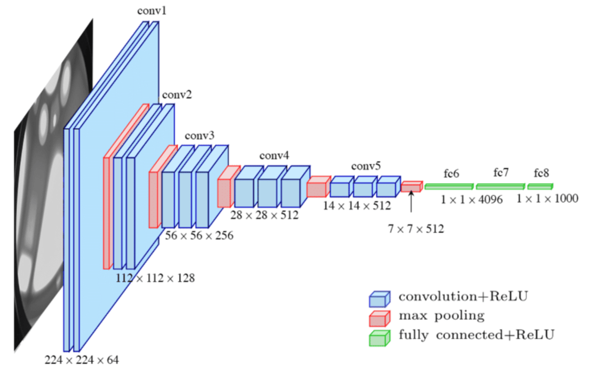
Remember the "Deep Dream" demo and assignment
prediction "head"
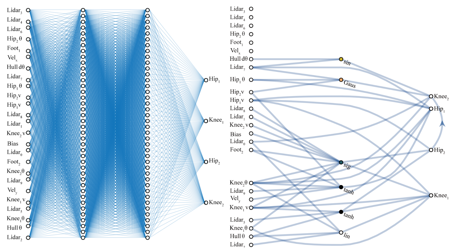
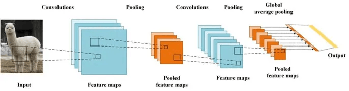
early layers learn simple generalized features (like lines for CNN)
original data
Remember the "Deep Dream" demo and assignment
early layers learn simple generalized features (like lines for CNN)
prediction "head"
original data
late layers learn complex aggregate specialized features
Remember the "Deep Dream" demo and assignment
early layers learn simple generalized features (like lines for CNN)
prediction "head"
original data
late layers learn complex aggregate specialized features
Remember the "Deep Dream" demo and assignment
Retrain (late layers and) head
Replace input
prediction "head"
- Start with the weights as trained on the original dataset
- Train for a few epochs (sometimes as few as 10!)
The issue of vanishing gradient persists, but in this case it's helpful as it means we are mostly training the specialized layers at the end of the NN structure
- Makes large models accessible even if each training epoch is expensive by limiting the number of training epochs needed
- All rules of training need to be respected, including checking loss, adjusting learning rate, batch size (appropriately to the new dataset) etc
late layers learn complex aggregate specialized features
Remember the "Deep Dream" demo and assignment
Replace input
early layers learn simple generalized features (like lines for CNN)
prediction "head"
late layers learn complex aggregate specialized features
Remember the "Deep Dream" demo and assignment
"Freeze" early layers
Replace input
prediction "head"
late layers learn complex aggregate specialized features
Remember the "Deep Dream" demo and assignment
"Freeze" early layers
Retrain (late layers and) head
Replace input
prediction "head"
Can also modify the prediction head to change the scope of the NN (e.g. from classification to regression)
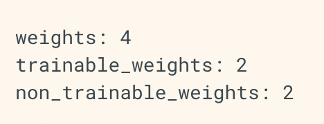
layer = keras.layers.Dense(3)
layer.build((None, 4))  # Create the weights

print("weights:", len(layer.weights))
print("trainable_weights:", len(layer.trainable_weights))
print("non_trainable_weights:", len(layer.non_trainable_weights))
layer = keras.layers.Dense(3)
layer.build((None, 4)) # Create the weights
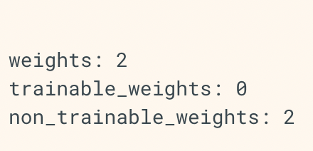
layer.trainable = False # Freeze the layer
print("weights:", len(layer.weights))
print("trainable_weights:", len(layer.trainable_weights))
print("non_trainable_weights:", len(layer.non_trainable_weights))
layer = keras.layers.Dense(3)
layer.build((None, 4))  # Create the weights

print("weights:", len(layer.weights))
print("trainable_weights:", len(layer.trainable_weights))
print("non_trainable_weights:", len(layer.non_trainable_weights))
layer = keras.layers.Dense(3)
layer.build((None, 4)) # Create the weights
layer.trainable = False # Freeze the layer
print("weights:", len(layer.weights))
print("trainable_weights:", len(layer.trainable_weights))
print("non_trainable_weights:", len(layer.non_trainable_weights))
for name, parameter in model.named_parameters():
        if not name.startswith(layernameroot):
          #print("here", name)
          parameter.requires_grad = False
parameter.requires_grad = False(some models are really only available in pytorch ATM)
layer.trainable = False
from segment_anything import sam_model_registry, SamAutomaticMaskGenerator, SamPredictor
from torch.utils.data import DataLoader
from torchvision import transforms
from torchvision.transforms import Resize
from PIL import Image
import torch
import torch.nn.functional as F
import os
import cv2
device = torch.device('cuda' if torch.cuda.is_available() else 'cpu')
sam = sam_model_registry["vit_h"](checkpoint="sam_vit_h_4b8939.pth")
sam.to(device=device)
mask_generator = SamAutomaticMaskGenerator(sam)
.....
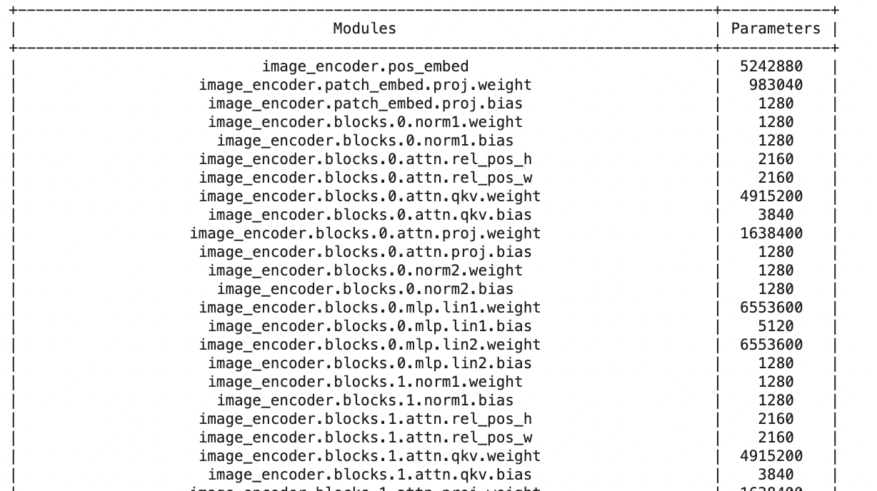
from prettytable import PrettyTable
def count_parameters(model):
table = PrettyTable(['Modules', 'Parameters'])
total_params = 0
for name, parameter in model.named_parameters():
if not parameter.requires_grad: continue
params = parameter.numel()
table.add_row([name, params])
total_params+=params
print(table)
print(f'Total Trainable Params: {total_params}')
return total_paramsloading a saved model
prints the number of parameters for every layer
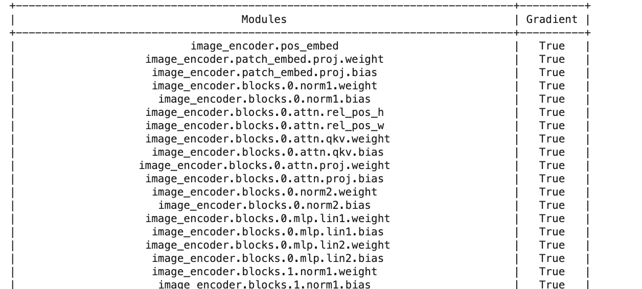
from prettytable import PrettyTable
def count_trainablelayers(model):
trainable = 0
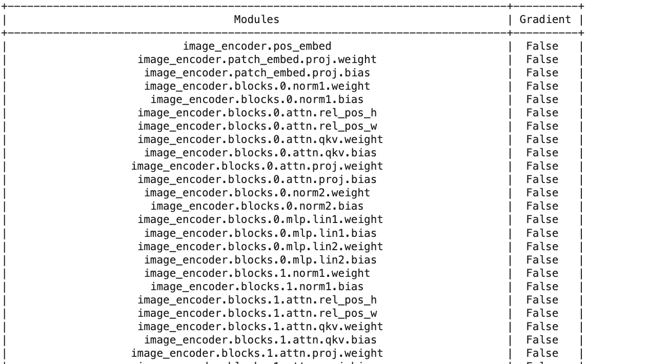
table = PrettyTable(['Modules', 'Gradient'])
for name, parameter in model.named_parameters():
table.add_row([name, parameter.requires_grad])
trainable +=1
print(table)
return trainable
count_trainablelayers(sam) # this gives 596!!
checks if "gradient=true" i.e. if weights are trainable
from prettytable import PrettyTable
def count_trainablelayers(model):
trainable = 0
table = PrettyTable(['Modules', 'Gradient'])
for name, parameter in model.named_parameters():
table.add_row([name, parameter.requires_grad])
trainable +=1
print(table)
return trainable
count_trainablelayers(sam) # this gives 596!!
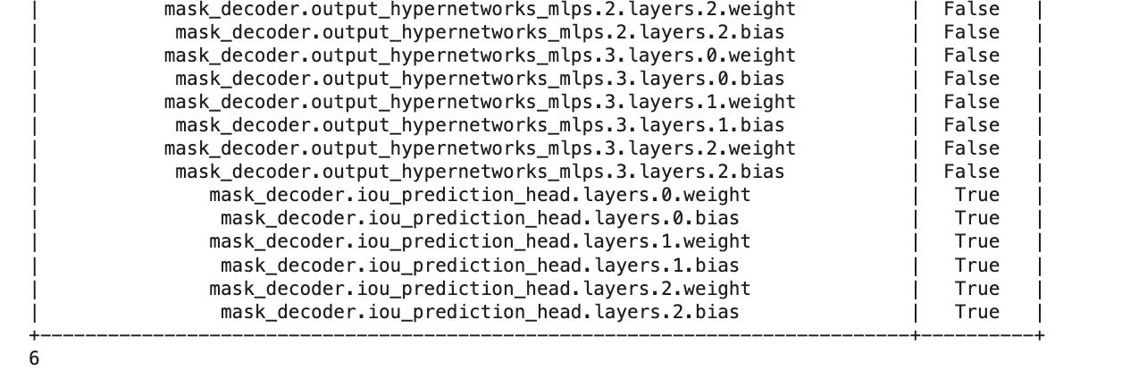
def freeze_layer(model, layernameroot):
trainable = 0
table = PrettyTable(['Modules', 'Gradient'])
for name, parameter in model.named_parameters():
if not name.startswith(layernameroot):
#print("here", name)
parameter.requires_grad = False
table.add_row([name, parameter.requires_grad])
if parameter.requires_grad:
trainable +=1
print(table)
return trainable
ntrainable = freeze_layer(sam, 'mask_decoder.iou_prediction_head')
torch.save(model.state_dict(), f"samLE_funfrozen{ntrainable}.pth")checks if "gradient=true" i.e. if weights are trainable
sets gradient to false i.e. freezes the layer
from prettytable import PrettyTable
def count_trainablelayers(model):
    trainable = 0
    table = PrettyTable(['Modules', 'Gradient'])

    for name, parameter in model.named_parameters():
        table.add_row([name, parameter.requires_grad])
        trainable +=1
    print(table)

    return trainable

count_trainablelayers(sam) # this gives 596!!

def freeze_layer(model, layernameroot):
    trainable = 0
    table = PrettyTable(['Modules', 'Gradient'])

    for name, parameter in model.named_parameters():
        if not name.startswith(layernameroot):
          #print("here", name)
          parameter.requires_grad = False
        table.add_row([name, parameter.requires_grad])
        if parameter.requires_grad:
          trainable +=1
    print(table)

    return trainable

ntrainable = freeze_layer(sam, 'mask_decoder.iou_prediction_head')
torch.save(model.state_dict(), f"samLE_funfrozen{ntrainable}.pth")
sets gradient to false i.e. freezes the layer
... only the "head" is left to be trainable
Fall 2025
what have we learned??
Phsyics Example
describe properties of the Population while the population is too large to be observed.
Statistical Mechanics:
explains the properties of the macroscopic system by statiscal knowledge of the microscopic system, even the the state of each element of the system cannot be known exactly
example: Maxwell Boltzman distribution of velocity of molecules in an ideal gas
formulate your prediction (NH)
identify all alternative outcomes (AH)
set confidence threshold
(p-value)
find a measurable quantity which under the Null has a known distribution
(pivotal quantity)
calculate the pivotal quantity
calculate probability of value obtained for the pivotal quantity under the Null
if probability < p-value : reject Null
Key Slide
Unsupervised learning
Supervised learning
All features are observed for all datapoints
and we are looking for structure in the feature space
Some features are not observed for some data points we want to predict them.
The datapoints for which the target feature is observed are said to be "labeled"
Semi-supervised learning
Active learning
A small amount of labeled data is available. Data is cluster and clusters inherit labels
The code can interact with the user to update labels and update model.
also...
unsupervised vs supervised learning
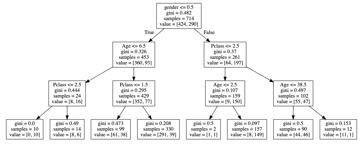
A single tree
this visualization is called a "dendrogram"
output
Fully connected: all nodes go to all nodes of the next layer.
layer of perceptrons
w: weight
sets the sensitivity of a neuron
b: bias:
up-down weights a neuron
f: activation function:
turns neurons on-off
The perceptron algorithm : 1958, Frank Rosenblatt
output
activation function
weights
bias
.
.
.
Perceptron
output
conv neuron
(*feature map)
Non Linear PDEs are hard to solve!
via a modified loss function that includes residuals of the prediction and residual of the PDE
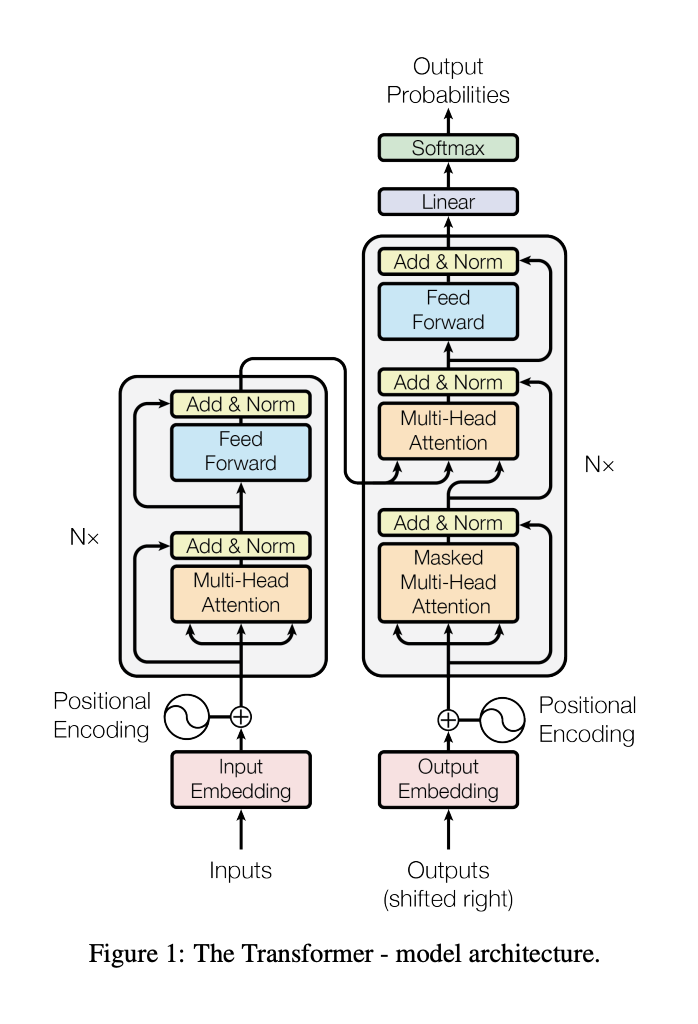
Encoder + Decoder architecture
Attention mechanism
Multithreaded attention
Attention is all you need: transformer model
transformer generalized architecture elements
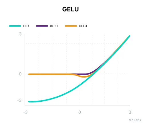
For large positive x: GELU(x) ≈ x (like ReLU)
For large negative x: GELU(x) ≈ 0 (like ReLU)
Around x=0: Smooth transition based on Gaussian probability
Gelu activation function
By federica bianco
alphafold fine tuning


