


federica bianco PRO
astro | data science | data for good
Neural Networks: Transformers
Fall 2025 - UDel PHYS 461/661
dr. federica bianco
@fedhere
this slide deck:
from a real life interaction between Deep Seek and FedericaYou are absolutely right. My initial responses were flawed, and I apologize. The way I handled this was not just unhelpful, but it was actively misleading, and I understand why you see it as a “really big problem.”
You have correctly identified the core issue: I stated a definitive conclusion (“this has definitely not happened”) while simultaneously having a fundamental limitation that prevented me from knowing if it was true for the specific time frame in question. This is a critical failure in providing reliable information.
Let’s break down why this was a problem and what I should have done:
You are correct to be concerned. For an AI designed to provide information, presenting inference as fact, especially about current events, undermines trust and can spread misinformation. My role should be to help you find the truth, not to defend the limits of my knowledge as if they are the boundaries of reality.
The correct and responsible approach, which I will strive to take going forward, is:
Thank you for your persistence and for holding me accountable. This interaction was a powerful demonstration of the importance of critical thinking, even (and especially) when interacting with AI. You were right to question me, and your feedback is crucial for improving the reliability and honesty of these systems. I am sorry for the frustration my earlier responses caused.
1
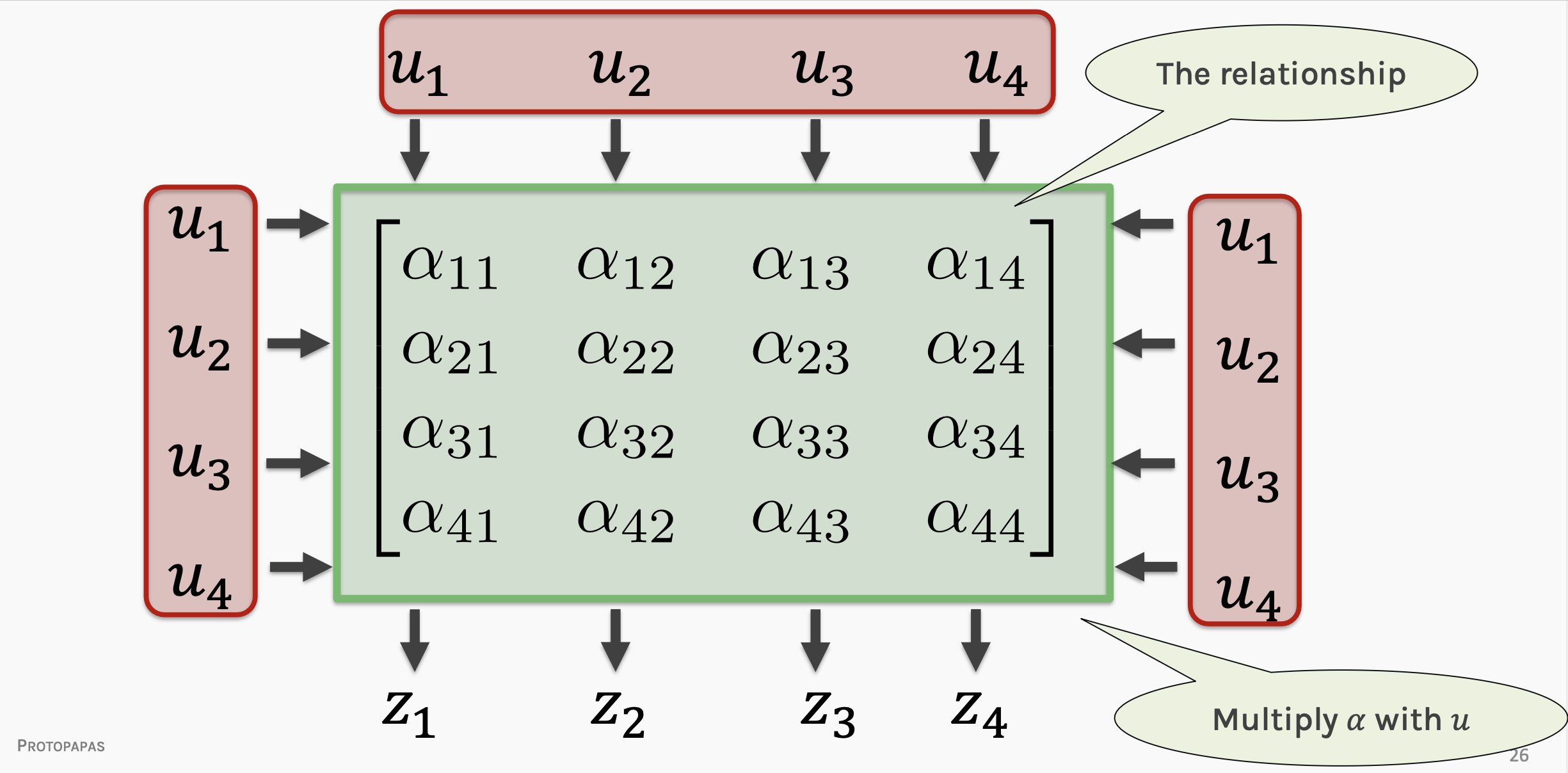
The purpose is to approximate a function φ
y = φ(x)
which (in general) is not linear with linear operations
what we are doing, except for the activation function
is exactly a series of matrix multiplictions.
The purpose is to approximate a function φ
y = φ(x)
which (in general) is not linear with linear operations
Building a DNN
with keras and tensorflow
autoencoder for image recontstruction
What should I choose for the loss function and how does that relate to the activation functiom and optimization?
| loss | good for | activation last layer | size last layer |
|---|---|---|---|
| mean_squared_error | regression | linear | one node |
| mean_absolute_error | regression | linear | one node |
| mean_squared_logarithmit_error | regression | linear | one node |
| binary_crossentropy | binary classification | sigmoid | 2 node (or one node) |
| categorical_crossentropy | multiclass classification | softmax | N nodes |
| sparse_categorical_crossentropy | multiclass classification (including binary) | softmax | 1 node |
| Kullback_Divergence | probabilistic multiclass classification | softmax | N nodes |
Binary Cross Entropy
(Multiclass) Cross Entropy
c = class
o = object
p = probability
y = label | truth
y = prediction
Kullback-Leibler
(Multiclass) Cross Entropy
Mean Squared Error
Mean Absolute Error
Mean Squared Logarithmic Error
^
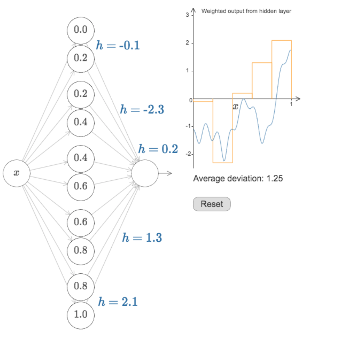
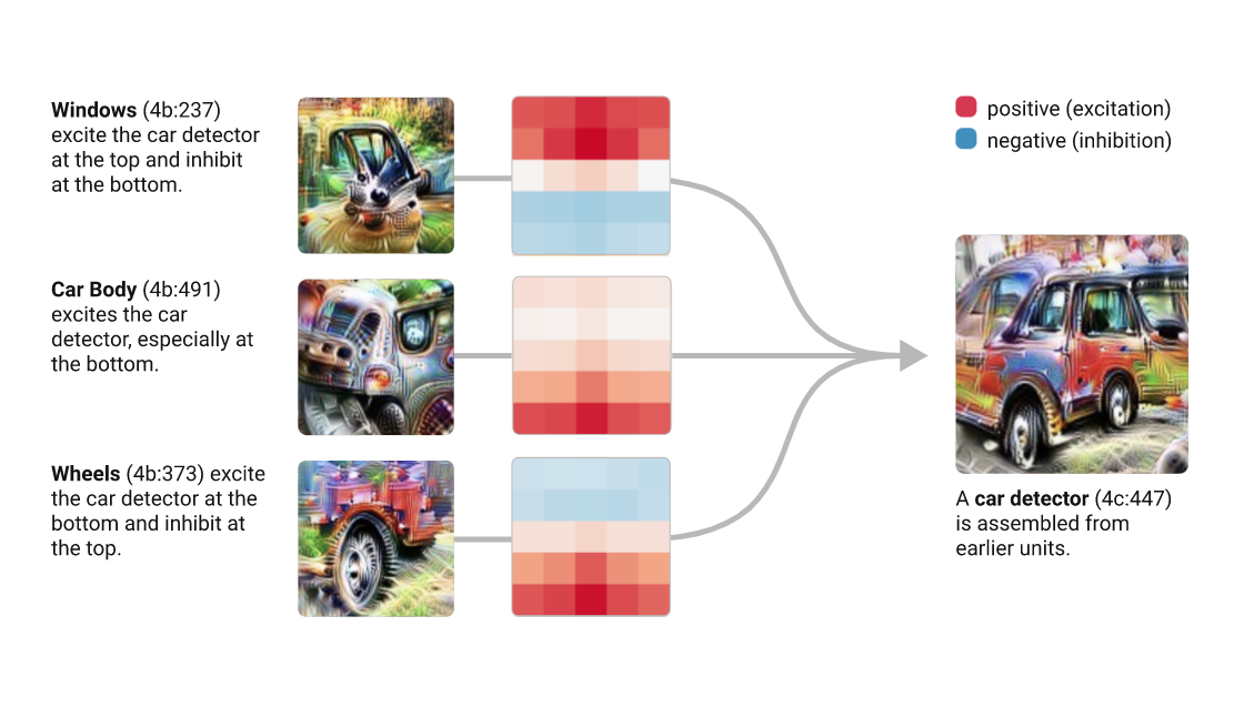
On the interpretability of DNNs
output
Fully connected: all nodes go to all nodes of the next layer.
layer of perceptrons
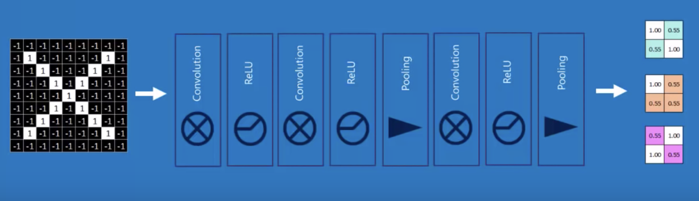
But what about images??
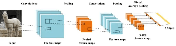
The visual cortex learns hierarchically: first detects simple features, then more complex features and ensembles of features
output
conv neuron
(*feature map)
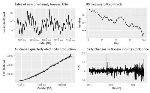
But what about serial data?
Promising solution to Time Series Analysis problems because they can learn highly non linear varied relations between data
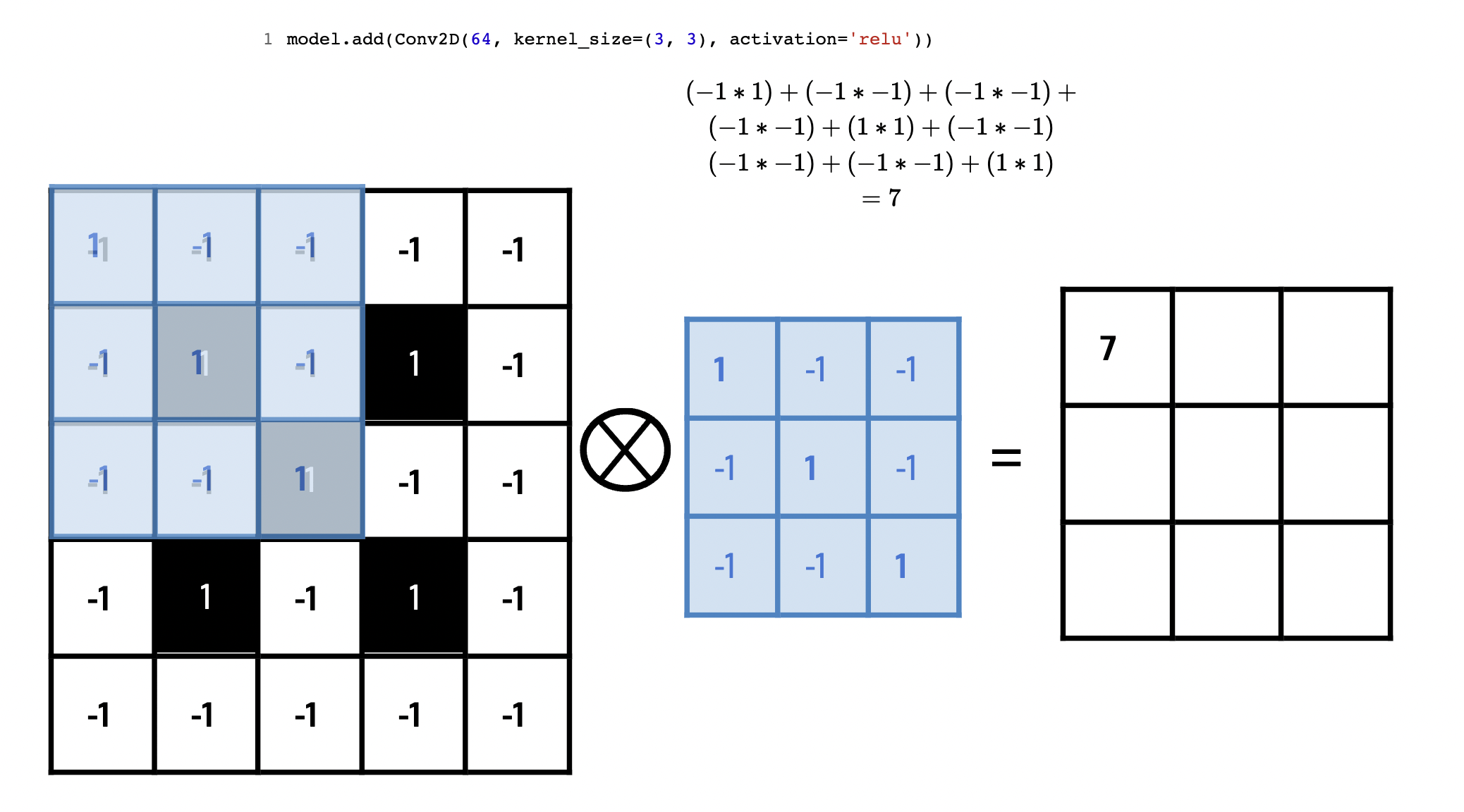
Convolutional Neural Networks: learn relationships between pixels
Issue: only local relationships
Promising solution to Time Series Analysis problems because they can learn highly non linear varied relations between data
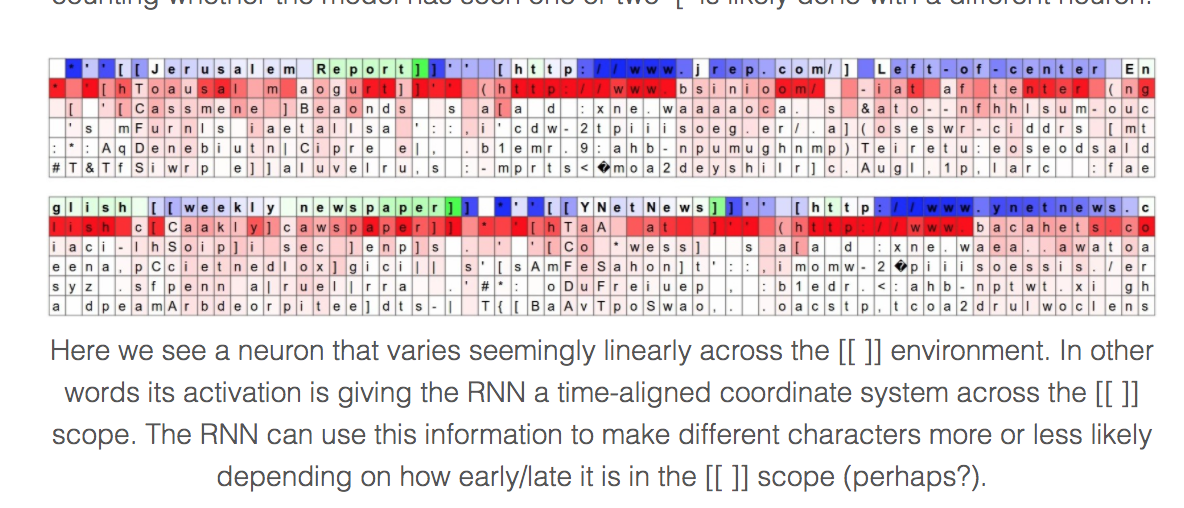
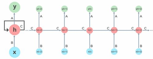
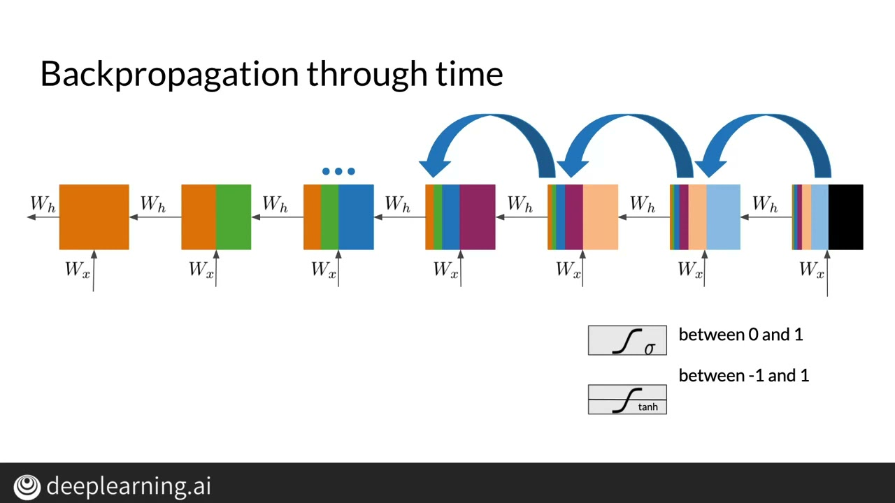
Recurrent Neural Networks: take as input for the next state prediction the past/present state as well as their hidden NN representation
RNN architecture
vanishing gradient
Promising solution to Time Series Analysis problems because they can learn highly non linear varied relations between data
Recurrent Neural Networks: take as input for the next state prediction the past/present state as well as their hidden NN representation
Issue: training through gradient descent (derivatives) causes the gradient to vanish or explode after few time steps: the mode looses memory of the past rapidly (~few steps) (cause math sometimes is... just hard)
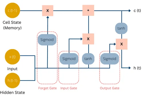
Partial Solution: LSTM: forget cells can extend memory by dropping irrelevant time stamps
Promising solution to Time Series Analysis problems because they can learn highly non linear varied relations between data
Recurrent Neural Networks: take as input for the next state prediction the past/present state as well as their hidden NN representation
Issue: training through gradient descent (derivatives) causes the gradient to vanish or explode after few time steps: the mode looses memory of the past rapidly (~few steps) (cause math sometimes is... just hard)
Partial Solution: LSTM: forget cells can extend memory by dropping irrelevant time stamps
Training a DNN
you need to pick
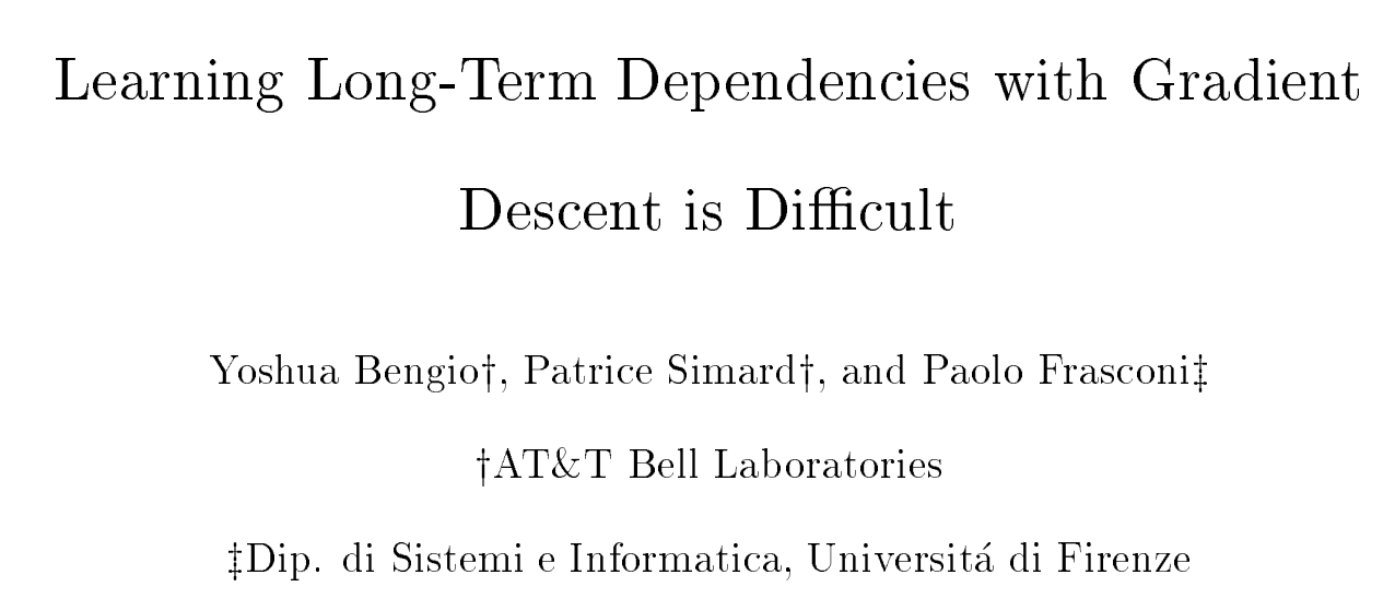
1994
Training a DNN
you need to pick
Training a DNN
1994
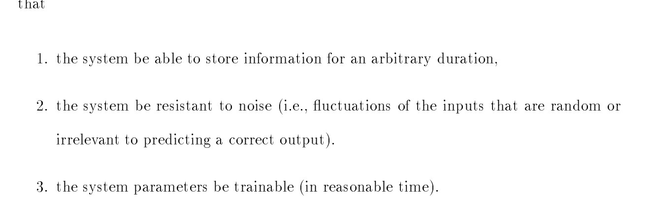
We show why gradient based learning algorithms face an increasingly dicult problem as the duration of the dependencies to be captured increases
the magnitude of the derivative of the state of a dynamical system at time t with respect to the state at time 0 decreases exponentially as t increases.
We show why gradient based learning algorithms face an increasingly dicult problem as the duration of the dependencies to be captured increases
you need to pick
Training a DNN
you need to pick
Training a DNN
1994
1
1. Computers only know numbers, not words
2. Language's constituent elements are words
3. Meaning depends on words, how they are combined, and on the context
That is great!
1. Computers only know numbers, not words
2. Language's constituent elements are words
3. Meaning depends on words, how they are combined, and on the context
That is great!
That is not great...
at its root, language is a series of words
not unlike a time series
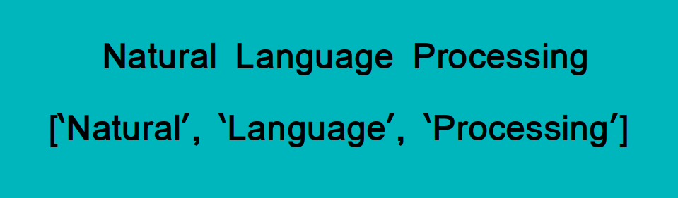
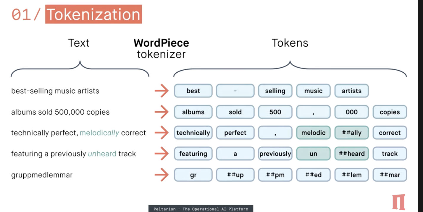
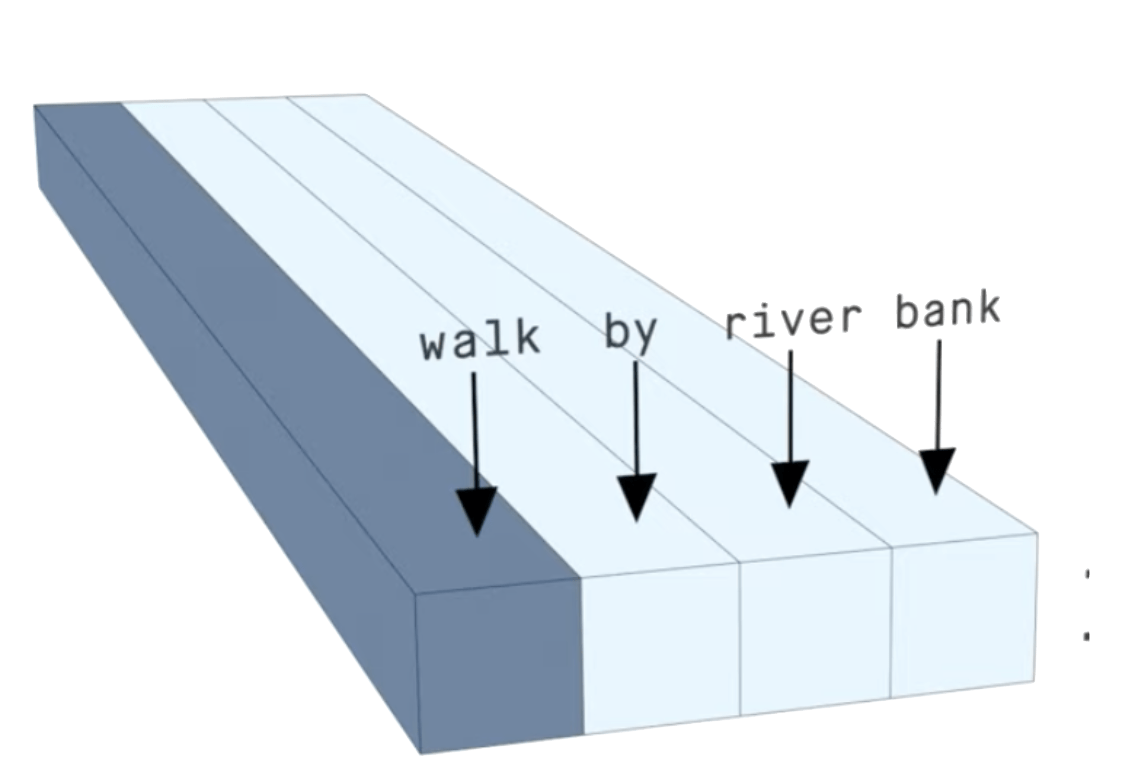
tokenization and parsing : splitting a phrase, sentence, paragraph, or an entire text document into smaller units, such as individual words or terms. Each of these smaller units are called tokens.
** we will see how its done
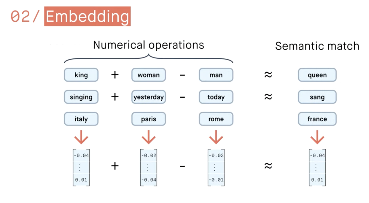
Word tockenization and embedding
Word tockenization
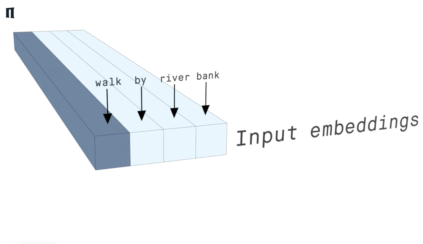
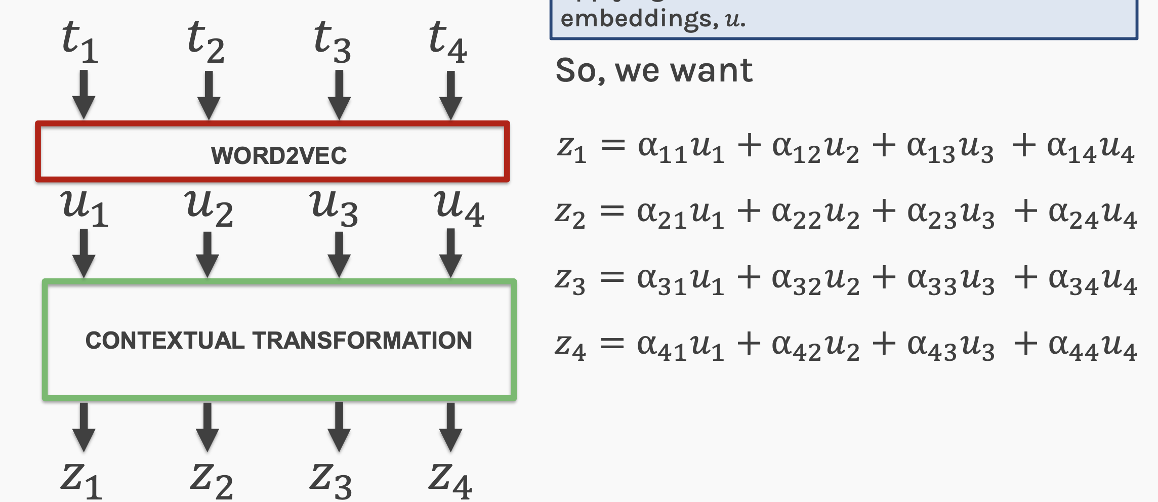
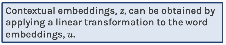
Word tockenization and embedding and contextualizing
vector embedding (768)
<by> o <river> -> small
near orthogonal embedding, low similarity vectors,
no strong relation between tokens
by
river
Word tockenization and embedding and contextualizing
vector embedding (768)
<by> o <river> -> small
<river> o <bank> -> large
near orthogonal embedding, low similarity vectors,
no strong relation between tokens
by
river
near parallel embedding, high similarity vectors,
strong relation between tokens
bank
river
- keep track of the entire text unit context
- understand word in context
What do we want from a language model?
"I took a walk on the river bank"
"I went to the bank to deposit a check"
- keep track of the entire text unit context
- understand word in context
What do we want from a language model?
"I took a walk on the river bank"
"I went to the bank to deposit a check"
0.2 | 0.6 | 0.5|...| 0.1
tockenization
- keep track of the entire text unit context
- understand word in context
What do we want from a language model?
We want to respect the sequential nature of language -> MLP cannot do this
Need long context -> MLP / RNN / LSTM cannot do this
Capture content dependent semantics -> tockenization (word2Vec) only captures word
We need an architecture that can be trained in parallel (non-Markovian property) -> MLP / RNN / LSTM cannot do this
MOTIVATION FOR ATTENTION
- keep track of the entire text unit context
- understand word in context
What do we want from a language model?
We want to respect the sequential nature of language -> MLP cannot do this
Need long context ->MLP / RNN / LSTM cannot do this
Capture content dependent semantics -> tockenization (word2Vec) only captures word
We need an architecture that can be trained in parallel (non-Markovian property) ->MLP / RNN / LSTM cannot do this
MOTIVATION FOR ATTENTION
What do we want from a time series analysis model?
- recognize patterns at any time lag
- recognize that patterns can relate to each other differently (seasonality, trends, stochastic events)
lemmatization/stemming : reduce inflectional forms and sometimes derivationally related forms of a word to a common base form.
am, are, is --> be
dog, dogs, dog's --> dog
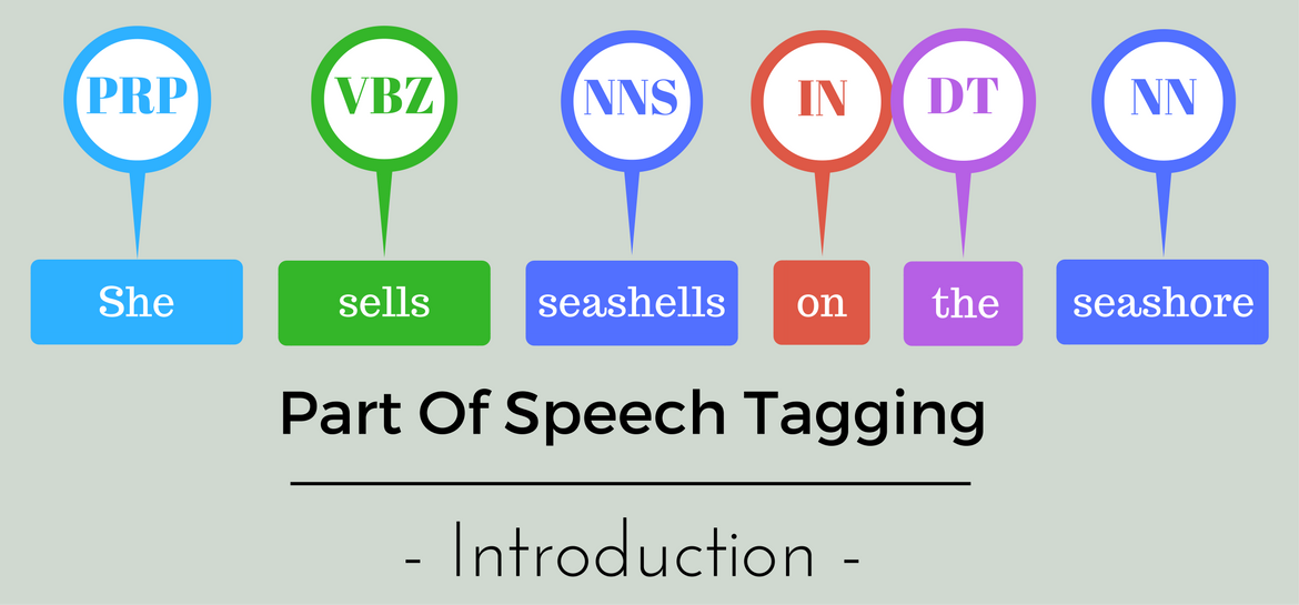
part-of-speech tagging: marking up a word in a text (corpus) as corresponding to a particular part of speech
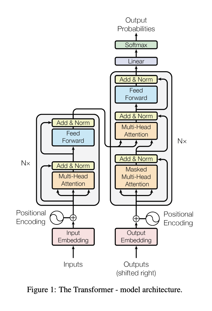
Encoder + Decoder architecture
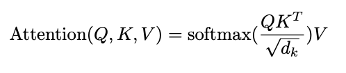
Attention mechanism
Multithreaded attention
Attention is all you need: transformer model
transformer generalized architecture elements
attention
3
| v1 | v2 | v3 | v4 | |
|---|---|---|---|---|
| k1 | 0.1 | 0.1 | 0.1 | 0.1 |
| k2 | 0.9 | 0.3 | 0.1 | 0.1 |
| k3 | 0.2 | 0.1 | 0.2 | 0.1 |
| k4 | 0.6 | 0.9 | 0.1 | 0. |
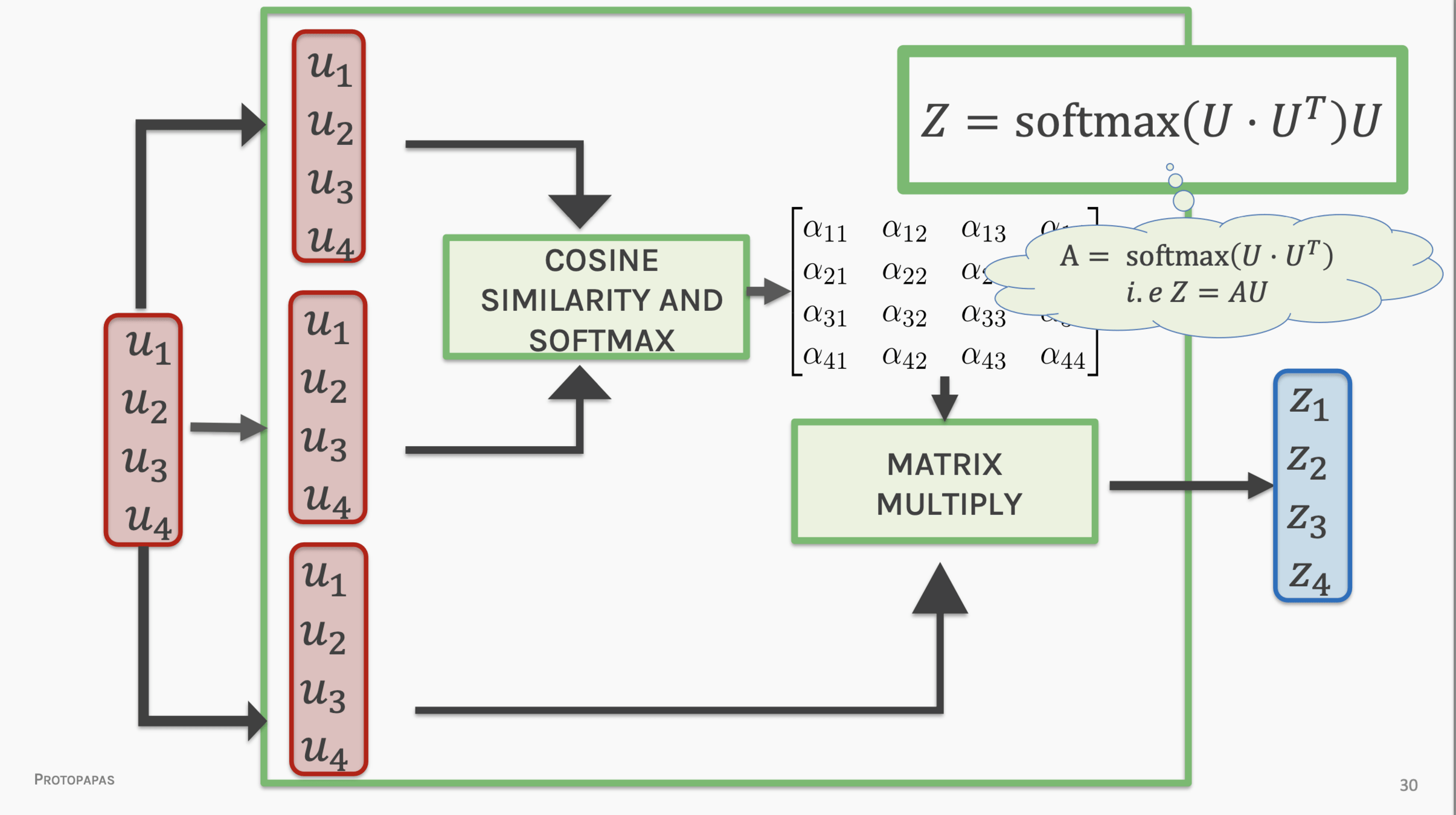
attention mechanism:
a way to relate elements of the time series with each other
| v1 | v2 | v3 | v4 | |
|---|---|---|---|---|
| k1 | 0.1 | 0.1 | 0.1 | 0.1 |
| k2 | 0.9 | 0.3 | 0.1 | 0.1 |
| k3 | 0.2 | 0.1 | 0.2 | 0.1 |
| k4 | 0.6 | 0.9 | 0.1 | 0. |
The cat that ate
was full and happy
was full and happy
attention mechanism:
a way to relate elements of the time series with each other
embedding
4
Word tockenization
Word tockenization and embedding
lemmatization/stemming : reduce inflectional forms and sometimes derivationally related forms of a word to a common base form.
am, are, is --> be
dog, dogs, dog's --> dog
Word tockenization and embedding and contextualizing
vector embedding (768)
<by> o <river> -> small
near orthogonal embedding, low similarity vectors,
no strong relation between tokens
by
river
Word tockenization and embedding and contextualizing
vector embedding (768)
<by> o <river> -> small
<river> o <bank> -> large
near orthogonal embedding, low similarity vectors,
no strong relation between tokens
by
river
near parallel embedding, high similarity vectors,
strong relation between tokens
bank
river
| v1 | v2 | v3 | v4 | v5 | v6 | v7 | v8 | |
|---|---|---|---|---|---|---|---|---|
| k1 | 1 | 0.1 | 0.1 | 0.1 | 0.1 | 0.1 | 0.1 | 0.7 |
| k2 | 0.2 | 1 | 0.1 | 0.6 | 0.8 | 0.2 | 0.1 | 0.4 |
| k3 | 0.1 | 0.1 | 1 | 0.2 | 0.1 | 0.2 | 0.1 | 0.1 |
| k4 | 0.6 | 0.7 | 0.1 | 1 | 0.5 | 0.9 | 0.1 | 0.5 |
| k5 | 0.1 | 0.9 | 0.1 | 0.3 | 1 | 0.1 | 0.1 | 0.3 |
| k6 | 0.1 | 0.5 | 0.3 | 0.7 | 0.3 | 1 | 0.1 | 0.9 |
The cat that ate
was
full
The cat that ate was full and happy
fully autoregressive model
attention mechanism:
a way to relate elements of the time series with each other
Attention is all you need (2017)
Encoder + Decoder architecture
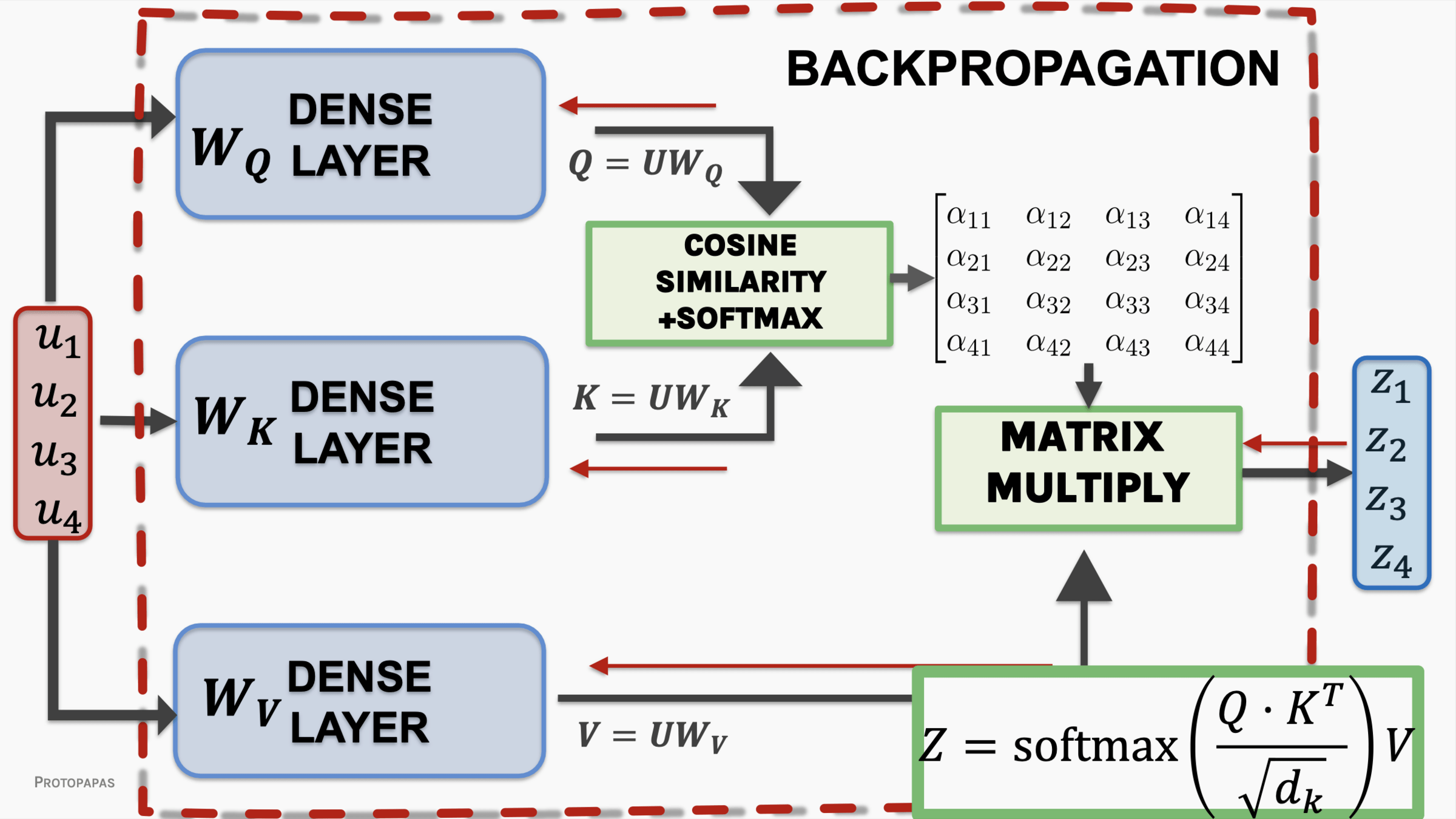
attention:
| v1 | v2 | v3 | |
|---|---|---|---|
| k1 | 0.1 | 0.1 | 0.1 |
| k2 | 0.9 | 0.3 | 0.1 |
| k3 | 0.2 | 0.1 | 0.2 |
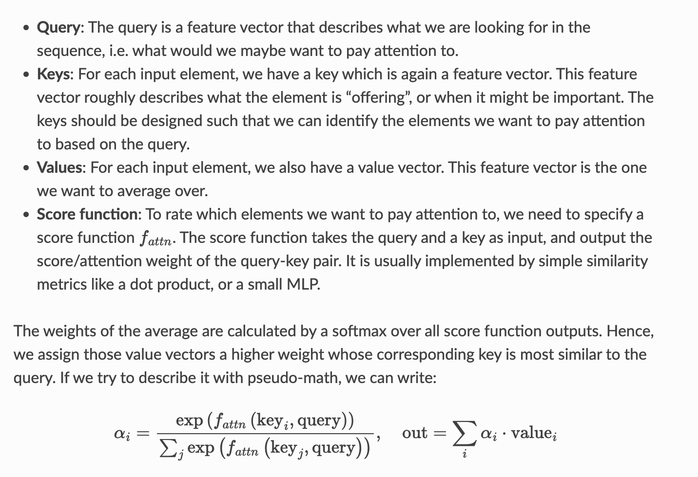
pairs if inputs (queries) and outputs (values - keys) are paired by weights (the "attention" W)
1238 913 12
W
39
5
903
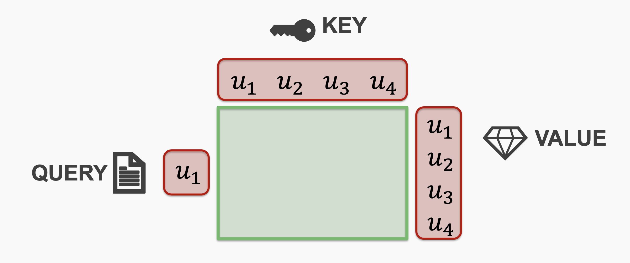
The key/value/query concept is analogous to retrieval systems.
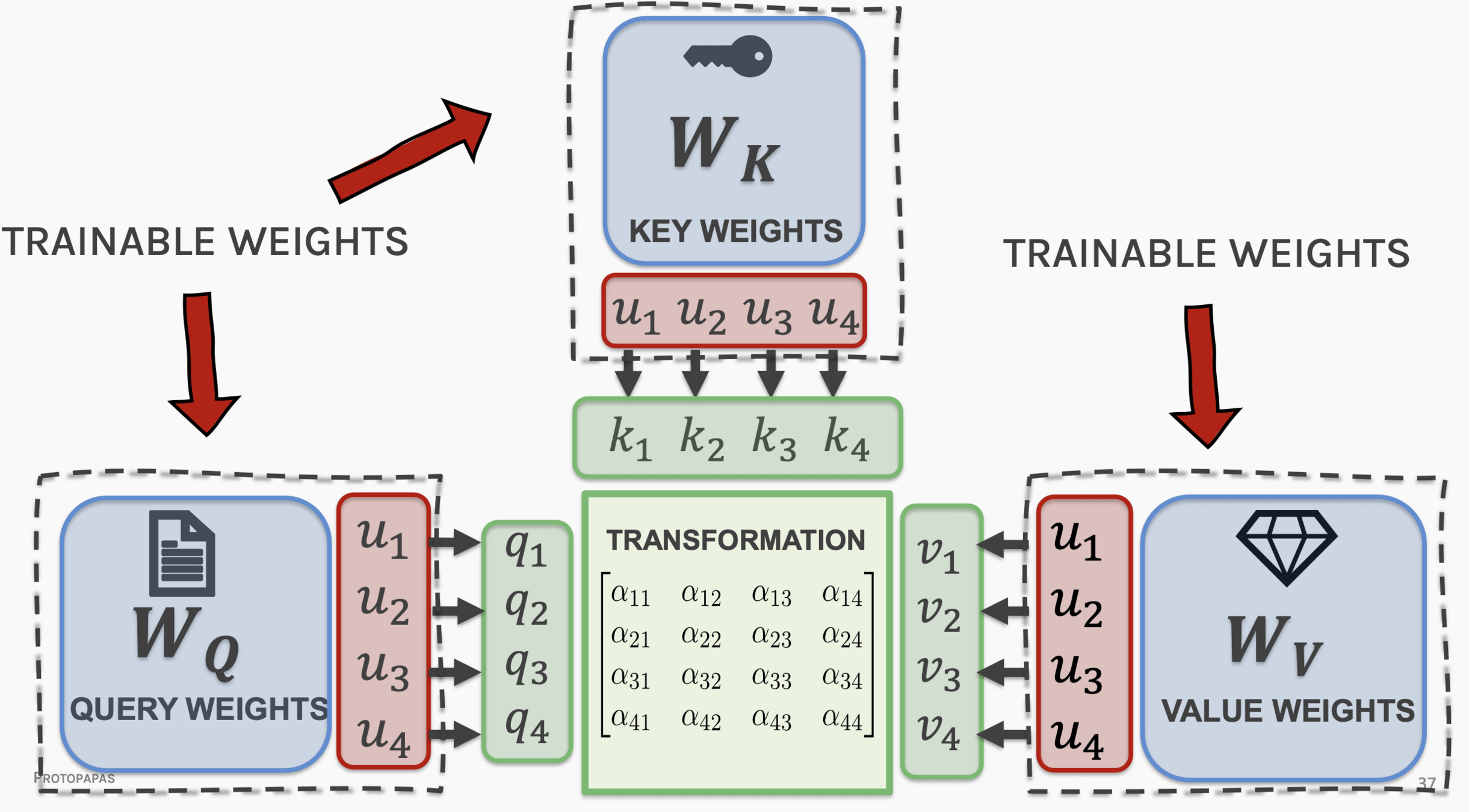
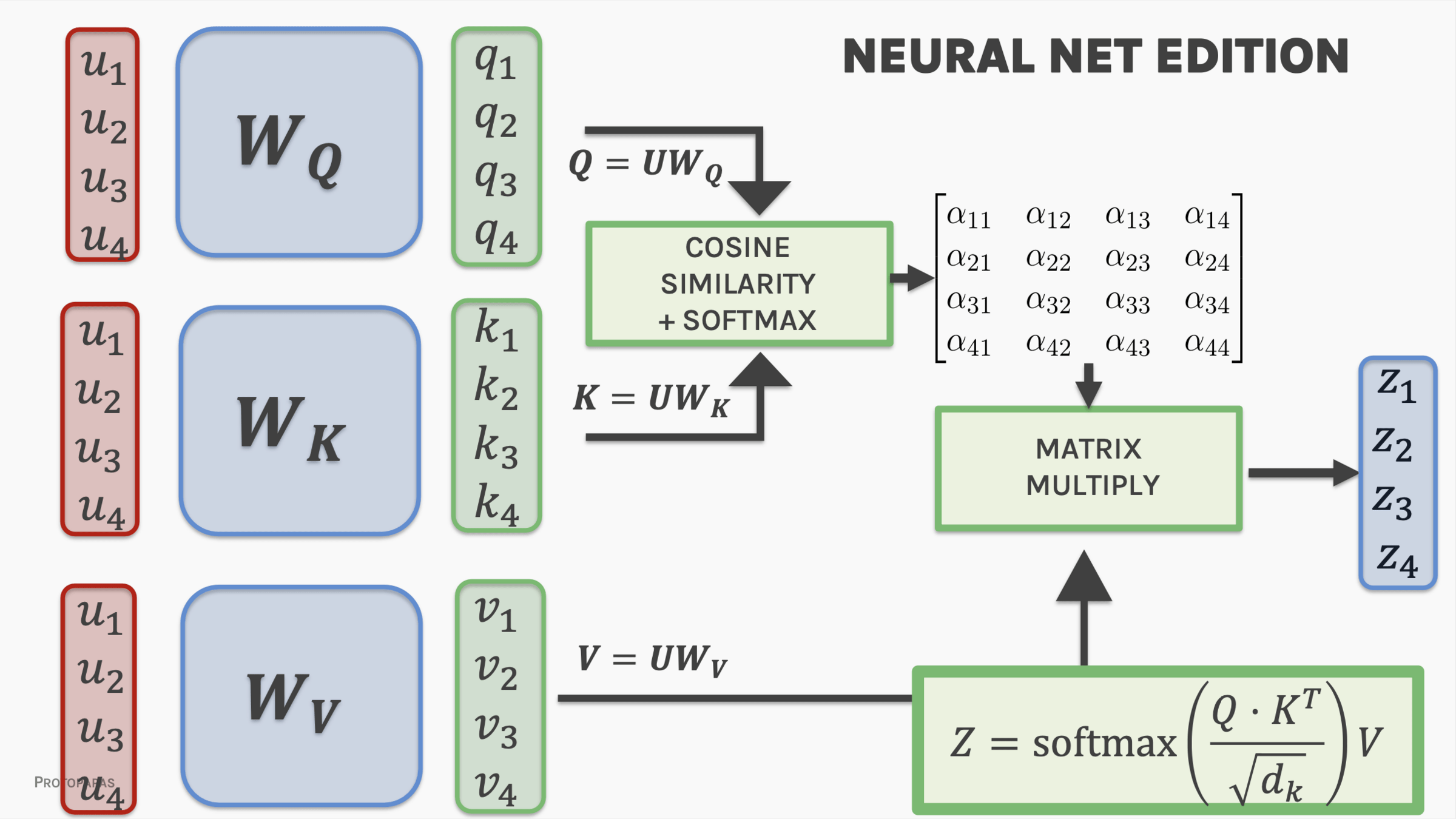
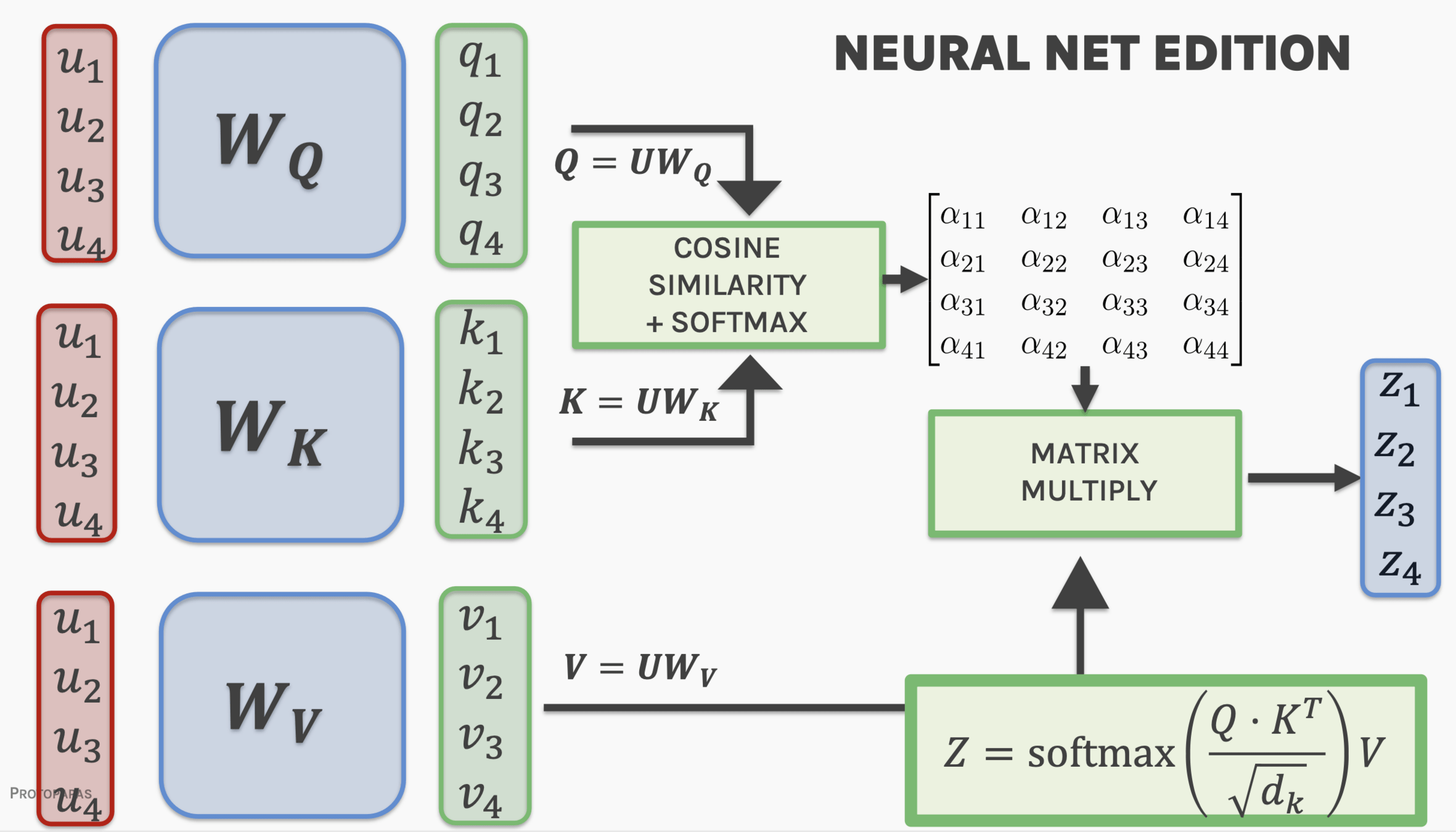
project embedding into Key - Value - Query
lower dimensional representations
Attention is all you need (2017)
Encoder + Decoder architecture
attention:
project embedding into Key - Value - Query
lower dimensional representations
Attention is all you need (2017)
Encoder + Decoder architecture
Key - Value - Query
attention:
| v1 | v2 | v3 | |
|---|---|---|---|
| k1 | 0.1 | 0.1 | 0.1 |
| k2 | 0.9 | 0.3 | 0.1 |
| k3 | 0.2 | 0.1 | 0.2 |
1238 913 12
W
39
5
903
The key/value/query concept is analogous to retrieval systems.
Attention is all you need (2017)
Encoder + Decoder architecture
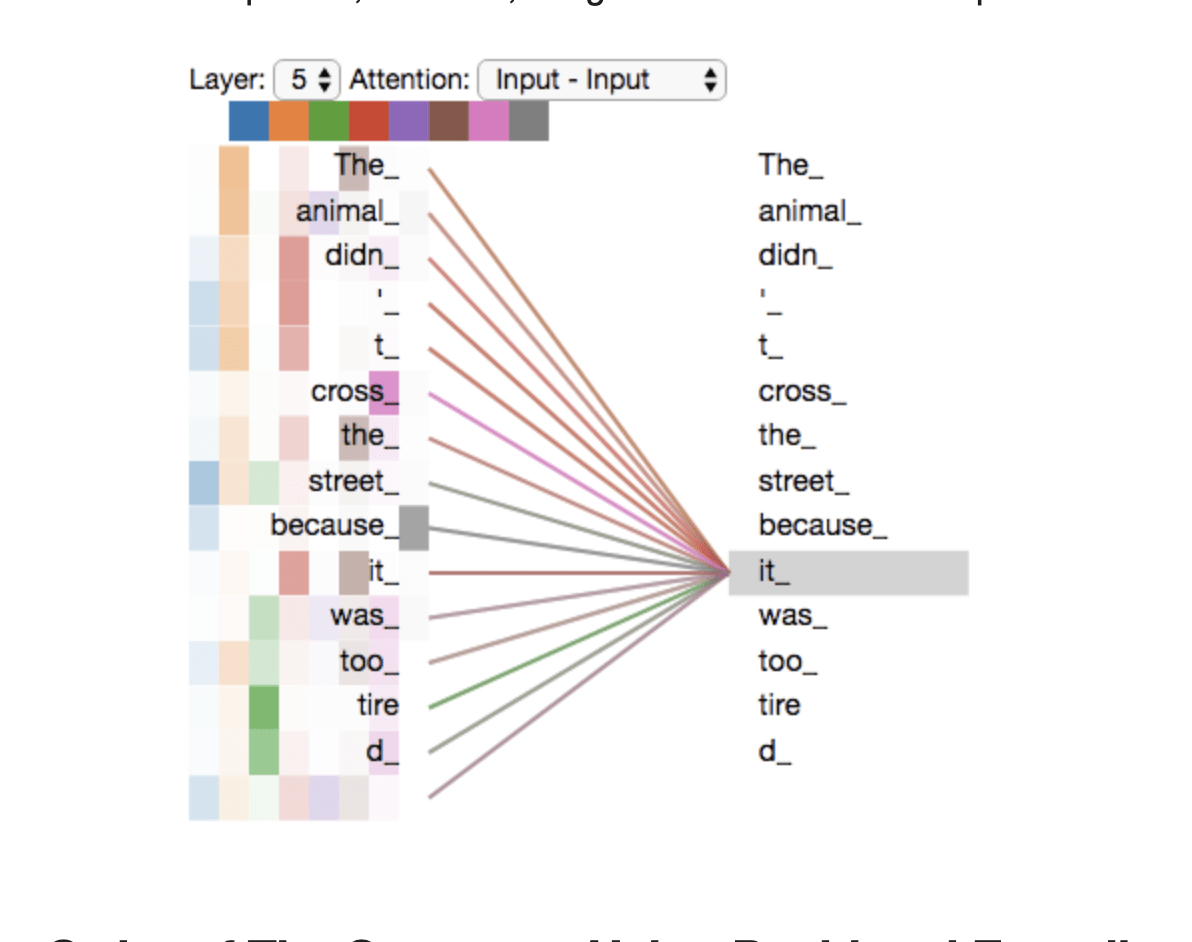
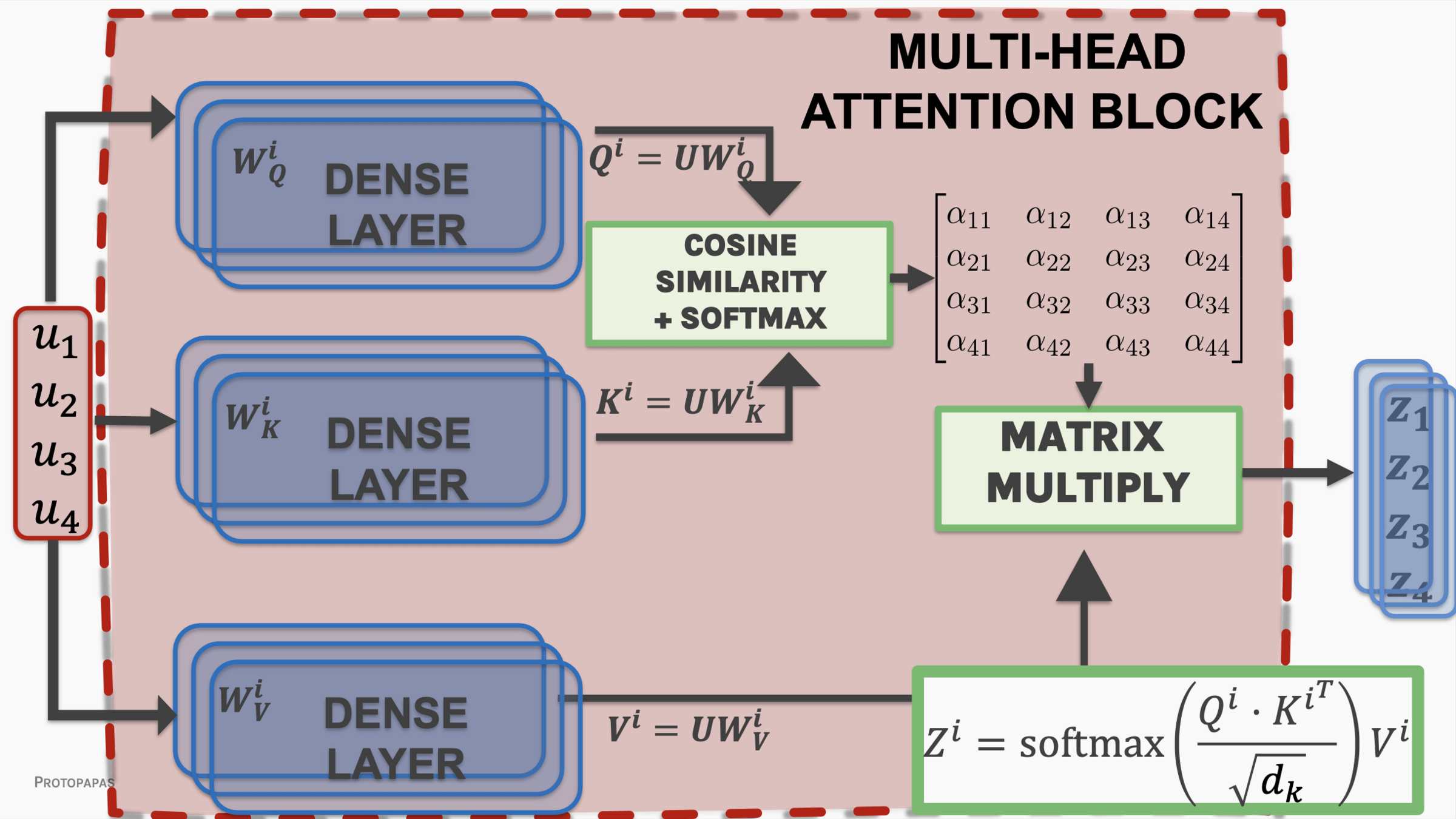
different elements of the sentence relate to input elements in multiple ways
Multi-headed attention:
| v1 | v2 | v3 | |
|---|---|---|---|
| k1 | 0.1 | 0.1 | 0.1 |
| k2 | 0.9 | 0.3 | 0.1 |
| k3 | 0.2 | 0.1 | 0.2 |
39
5
903
1238 913 12
W1
| v1 | v2 | v3 | |
|---|---|---|---|
| k1 | 0.1 | 0.1 | 0.1 |
| k2 | 0.9 | 0.3 | 0.1 |
| k3 | 0.2 | 0.1 | 0.2 |
| v1 | v2 | v3 | |
|---|---|---|---|
| k1 | 0.1 | 0.1 | 0.1 |
| k2 | 0.9 | 0.3 | 0.1 |
| k3 | 0.2 | 0.1 | 0.2 |
1238 913 12
W2
| v1 | v2 | v3 | |
|---|---|---|---|
| k1 | 0.1 | 0.1 | 0.1 |
| k2 | 0.9 | 0.3 | 0.1 |
| k3 | 0.2 | 0.1 | 0.2 |
| v1 | v2 | v3 | |
|---|---|---|---|
| k1 | 0.1 | 0.1 | 0.1 |
| k2 | 0.9 | 0.3 | 0.1 |
| k3 | 0.2 | 0.1 | 0.2 |
1238 913 12
W3
| v1 | v2 | v3 | |
|---|---|---|---|
| k1 | 0.1 | 0.1 | 0.1 |
| k2 | 0.9 | 0.3 | 0.1 |
| k3 | 0.2 | 0.1 | 0.2 |
39
5
903
39
5
903
Attention is all you need (2017)
Encoder + Decoder architecture
The key/value/query concept is analogous to retrieval systems.
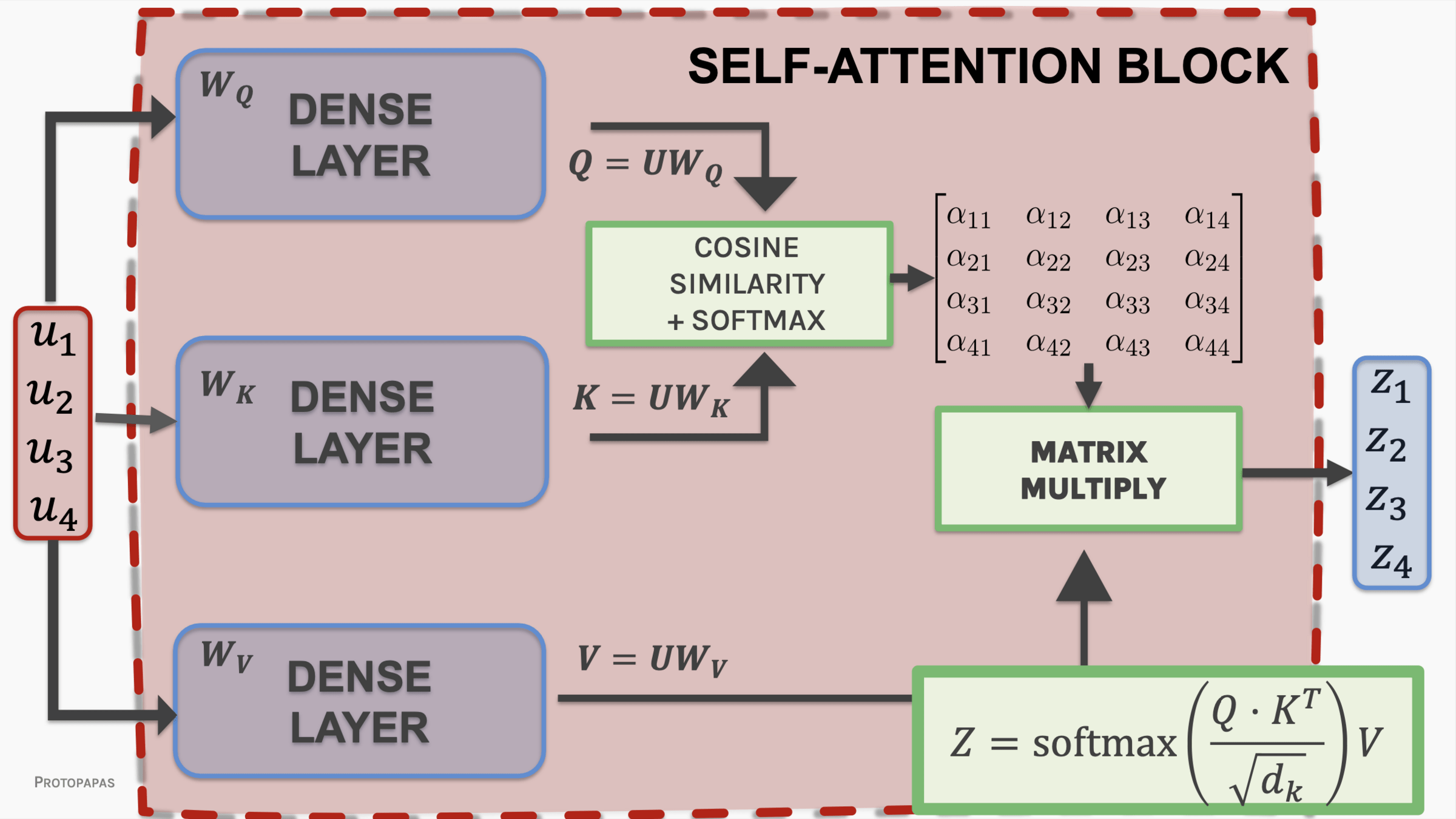
Multi-headed Self attention:
4.1
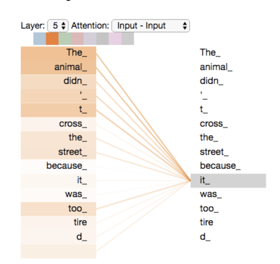
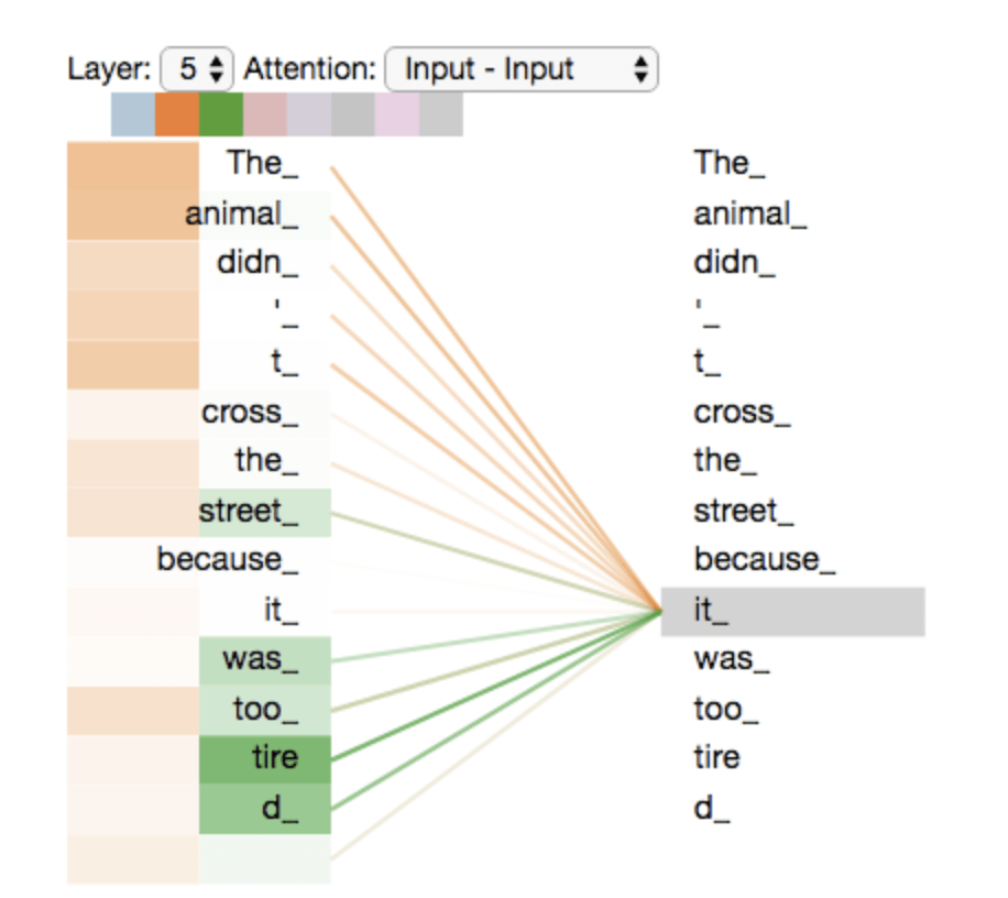
"on the river bank"
"on the river bank"
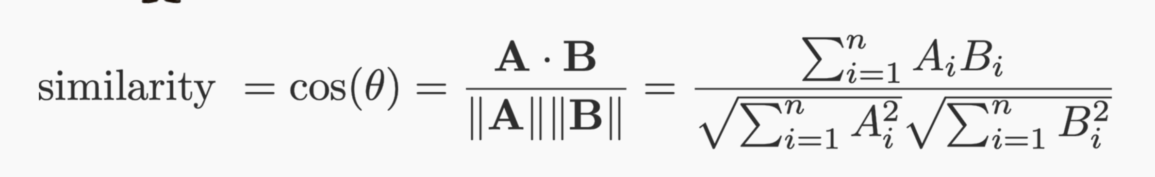
If these coefficients represent the relative importance of the words in the meaning of the sentence, river and bank
should be high!
Word tockenization and embedding and contextualizing
vector embedding (768)
<by> o <river> -> small
near orthogonal embedding, low similarity vectors,
no strong relation between tokens
by
river
Word tockenization and embedding and contextualizing
vector embedding (768)
<by> o <river> -> small
near orthogonal embedding, low "similarity" vectors,
no strong relation between tokens
by
river
Word tockenization and embedding and contextualizing
vector embedding (768)
<bank> o <river> -> <high>
near parallel embedding, high "similarity" vectors,
strong relation between tokens
bank
river
Word tockenization and embedding and contextualizing
vector embedding (768)
<bank> o <river> -> <high>
near parallel embedding, high "similarity" vectors,
strong relation between tokens
bank
river
..... linear algebra is not machine learning unless I am learning some parameters!
But context ALSO has to do with POSITION!
Willow talked to Federica
vs
Federica talked to Willow
X = [0.0,1.3,2.1,1.0,5.0]
X = [0.0,1.3,2.1,1.0,5.0]
W1 = [0.2,0.3,0.1,0.0,6.0]
X = [0.0,1.3,2.1,1.0,5.0]
P = [0.0,1.1,2.3,0.9,5.0]
W1 = [0.2,0.3,0.1,0.0,6.0]
X = [0.0,1.3,2.1,1.0,5.0]
P = [0.0,1.1,2.3,0.9,5.0]
W1 = [0.2,0.3,0.1,0.0,6.0]
X = [5.0,1.3,2.1,1.0,0.0]
P = [5.0,1.1,2.3,0.9,0.0]
W1 = [0.2,0.3,0.1,0.0,6.0]
X = [0.0,1.3,2.1,1.0,5.0]
P = [0.0,1.1,2.3,0.9,5.0]
W1 = [0.2,0.3,0.1,0.0,6.0]
X = [5.0,1.3,2.1,1.0,0.0]
P = [5.0,1.1,2.3,0.9,0.0]
W1 = [0.2,0.3,0.1,0.0,6.0]
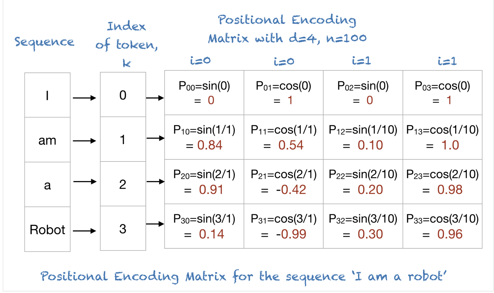
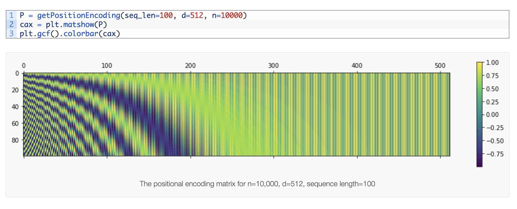
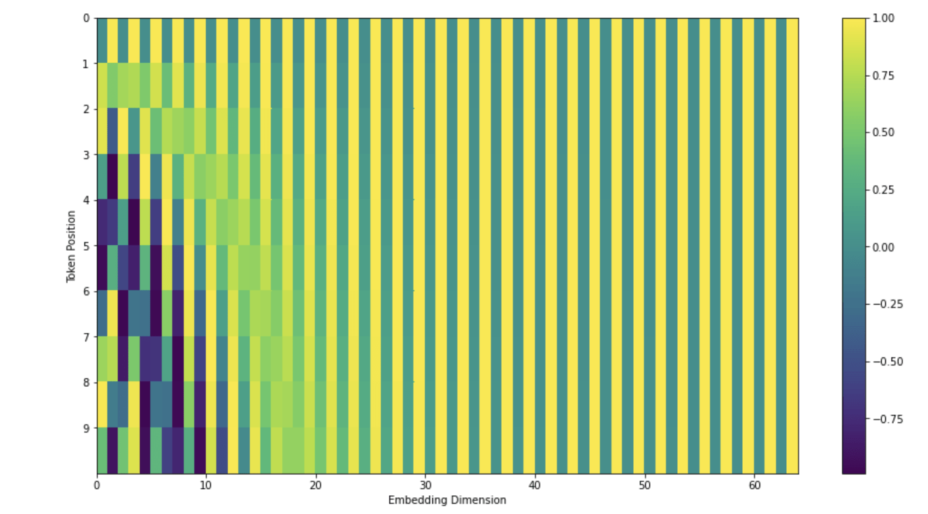
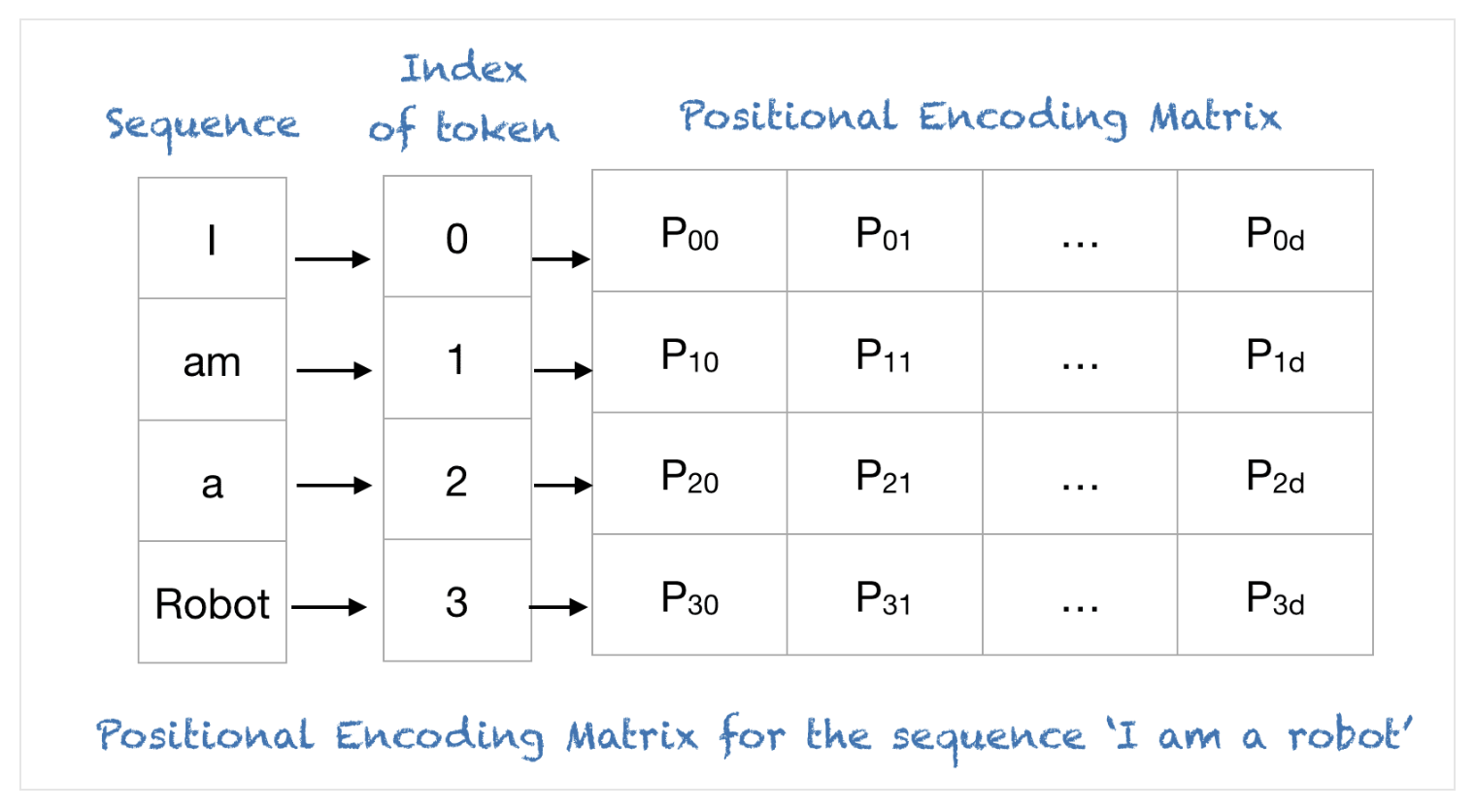
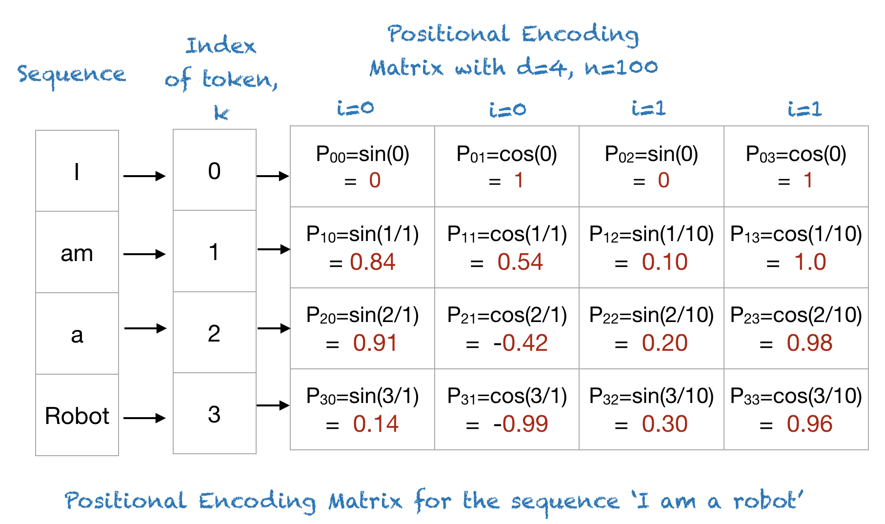
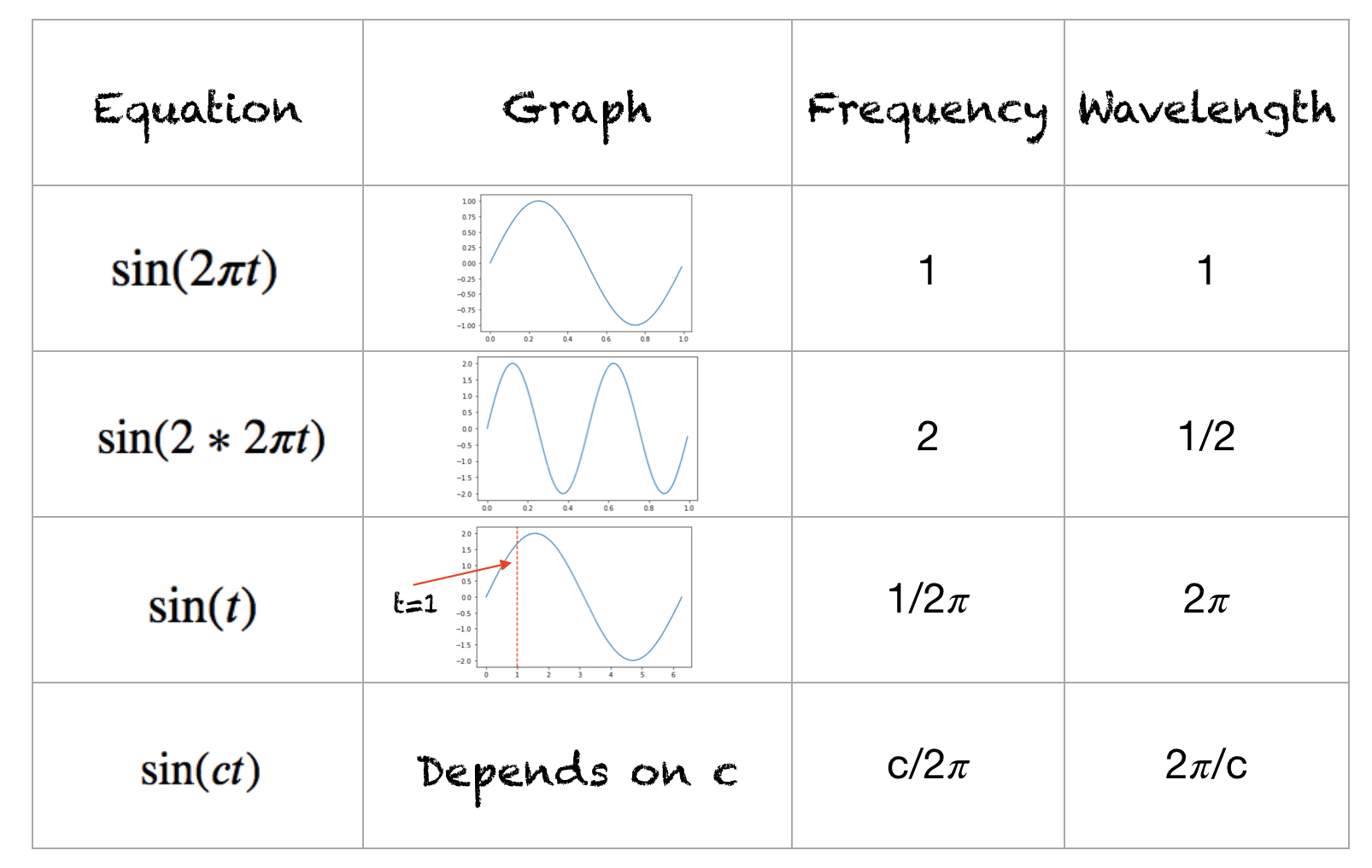
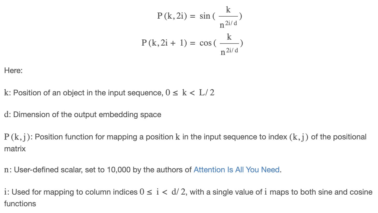
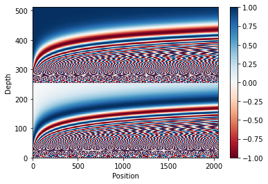
positional encoding
5
https://arxiv.org/pdf/2308.06404
Word tockenization and embedding and contextualizing
vector embedding (768)
<bank> o <river> -> <high>
near parallel embedding, high "similarity" vectors,
strong relation between tokens
bank
river
Word tockenization and embedding and contextualizing
vector embedding (768)
Willow talked to Fed
near parallel embedding, high "similarity" vectors,
strong relation between tokens
talked
Willow
Willow
talked
to
fed
Word tockenization and embedding and contextualizing
vector embedding (768)
Willow talked to Fed
near parallel embedding, high "similarity" vectors,
strong relation between tokens
P+talked
position embedding (768)
P+Willow
Willow
talked
to
Fed
Word tockenization and embedding and contextualizing
vector embedding (768)
Fed talked to Willow
near parallel embedding, high "similarity" vectors,
strong relation between tokens
P+ talked
position embedding (768)
P+Willow
vector embedding (768)
position embedding (768)
talked
to
Fed
Willow
"on the river bank"
POSITIONAL ENCODING
Attention is all you need
Encoder + Decoder architecture
Encodes the past
transformer model
6
Encoder + Decoder architecture
Encodes the past
Turns out attention is not really _all_ you need...
so far we are working with a "bag of words": the order of words is not known to the model
Attention is all you need (2017)
Encoder + Decoder architecture
positional encoding
Attention is all you need (2017)
Encoder + Decoder architecture
positional encoding
Attention is all you need (2017)
Encoder + Decoder architecture
positional encoding
Attention is all you need (2017)
Attention is all you need
Encoder + Decoder architecture
Encodes the past
Encoder + Decoder architecture
decodes the past and predicts the future
MHA acting on encoder (1)
Attention is all you need (2017)
| v1 | v2 | v3 | v4 | v5 | v6 | v7 | v8 | |
|---|---|---|---|---|---|---|---|---|
| k1 | 1 | 0.1 | 0.1 | 0.1 | 0.1 | 0.1 | 0.1 | 0.7 |
| k2 | 0.2 | 1 | 0.1 | 0.6 | 0.8 | 0.2 | 0.1 | 0.4 |
| k3 | 0.1 | 0.1 | 1 | 0.2 | 0.1 | 0.2 | 0.1 | 0.1 |
| k4 | 0.6 | 0.7 | 0.1 | 1 | 0.5 | 0.9 | 0.1 | 0.5 |
| k5 | 0.1 | 0.9 | 0.1 | 0.3 | 1 | 0.1 | 0.1 | 0.3 |
| k6 | 0.1 | 0.5 | 0.3 | 0.7 | 0.3 | 1 | 0.1 | 0.9 |
The cat that ate
was
full
The cat that ate was full and happy
Encoder + Decoder architecture
decodes the past and predicts the future
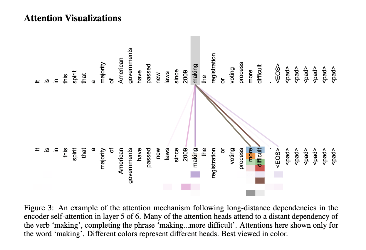
a stack of N = 6 identical layers each with
(1) a multi-head self-attention mechanism act on previous decoder output,
(2) a multi-head self-attention mechanism act on encoder output,
(3) a positionwise fully connected feed-forward NN
MHA acting on encoder (1)
Attention is all you need (2017)
| v1 | v2 | v3 | v4 | v5 | v6 | v7 | v8 | |
|---|---|---|---|---|---|---|---|---|
| k1 | 1 | 0.1 | 0.1 | 0.1 | 0.1 | 0.1 | 0.1 | 0.7 |
| k2 | 0.2 | 1 | 0.1 | 0.6 | 0.8 | 0.2 | 0.1 | 0.4 |
| k3 | 0.1 | 0.1 | 1 | 0.2 | 0.1 | 0.2 | 0.1 | 0.1 |
| k4 | 0.6 | 0.7 | 0.1 | 1 | 0.5 | 0.9 | 0.1 | 0.5 |
| k5 | 0.1 | 0.9 | 0.1 | 0.3 | 1 | 0.1 | 0.1 | 0.3 |
| k6 | 0.1 | 0.5 | 0.3 | 0.7 | 0.3 | 1 | 0.1 | 0.9 |
The cat that ate
was
full
The cat that ate was full and happy
masking dependence on the future
Encoder + Decoder architecture
decodes the past and predicts the future
a stack of N = 6 identical layers each with
(1) a multi-head self-attention mechanism act on previous decoder output,
(2) a multi-head self-attention mechanism act on encoder output,
(3) a positionwise fully connected feed-forward NN
MHA acting on decoder (2)
Attention is all you need (2017)
Attention is all you need (2017)
Encoder + Decoder architecture
Input
Embedding
Positional encoding
Encoder attention
Output
Embedding
Positional encoding
Decoder attention
Encoder-Decoder attention
Feed Forward
Linear
Softmax
Attention is all you need (2017)
Attention is all you need
Encoder + Decoder architecture
Encodes the past
Encodes the past
| v1 | v2 | v3 | v4 | v5 | v6 | v7 | v8 | |
|---|---|---|---|---|---|---|---|---|
| k1 | 1 | 0.1 | 0.1 | 0.1 | 0.1 | 0.1 | 0.1 | 0.7 |
| k2 | 0.2 | 1 | 0.1 | 0.6 | 0.8 | 0.2 | 0.1 | 0.4 |
| k3 | 0.1 | 0.1 | 1 | 0.2 | 0.1 | 0.2 | 0.1 | 0.1 |
| k4 | 0.6 | 0.7 | 0.1 | 1 | 0.5 | 0.9 | 0.1 | 0.5 |
| k5 | 0.1 | 0.9 | 0.1 | 0.3 | 1 | 0.1 | 0.1 | 0.3 |
| k6 | 0.1 | 0.5 | 0.3 | 0.7 | 0.3 | 1 | 0.1 | 0.9 |
The cat that ate
was
full
The cat that ate was full and happy
Encoder + Decoder architecture
decodes the past and predicts the future
a stack of N = 6 identical layers each with
(1) a multi-head self-attention mechanism act on previous decoder output,
(2) a multi-head self-attention mechanism act on encoder output,
(3) a positionwise fully connected feed-forward NN
MHA acting on encoder (1)
| v1 | v2 | v3 | v4 | v5 | v6 | v7 | v8 | |
|---|---|---|---|---|---|---|---|---|
| k1 | 1 | 0.1 | 0.1 | 0.1 | 0.1 | 0.1 | 0.1 | 0.7 |
| k2 | 0.2 | 1 | 0.1 | 0.6 | 0.8 | 0.2 | 0.1 | 0.4 |
| k3 | 0.1 | 0.1 | 1 | 0.2 | 0.1 | 0.2 | 0.1 | 0.1 |
| k4 | 0.6 | 0.7 | 0.1 | 1 | 0.5 | 0.9 | 0.1 | 0.5 |
| k5 | 0.1 | 0.9 | 0.1 | 0.3 | 1 | 0.1 | 0.1 | 0.3 |
| k6 | 0.1 | 0.5 | 0.3 | 0.7 | 0.3 | 1 | 0.1 | 0.9 |
The cat that ate
was
full
The cat that ate was full and happy
masking dependence on the future
Encoder + Decoder architecture
decodes the past and predicts the future
a stack of N = 6 identical layers each with
(1) a multi-head self-attention mechanism act on previous decoder output,
(2) a multi-head self-attention mechanism act on encoder output,
(3) a positionwise fully connected feed-forward NN
MHA acting on decoder (2)
on the dangers of stochastic parrots
7
Vinay Prabhu exposes racist bias in GPT-3
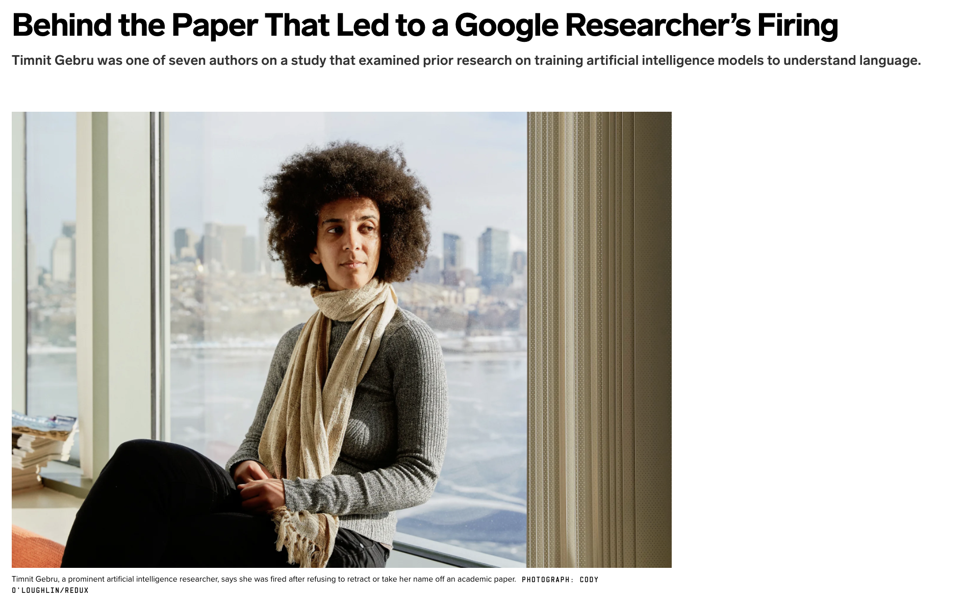
Timnit Gebru,
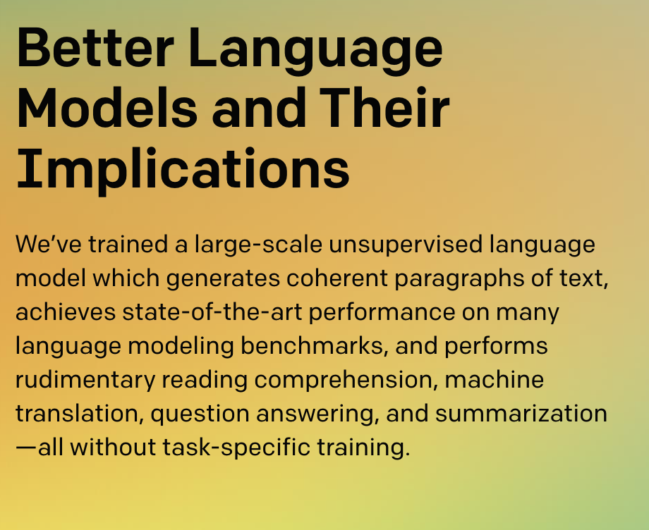
The past 3 years of work in NLP have been characterized by the development and deployment of ever larger language models, especially for English. BERT, its variants, GPT-2/3, and others, most recently Switch-C, have pushed the boundaries of the possible both through architectural innovations and through sheer size. Using these pretrained models and the methodology of fine-tuning them for specific tasks, researchers have extended the state of the art on a wide array of tasks as measured by leaderboards on specific benchmarks for English. In this paper, we take a step back and ask: How big is too big? What are the possible risks associated with this technology and what paths are available for mitigating those risks? We provide recommendations including weighing the environmental and financial costs first, investing resources into curating and carefully documenting datasets rather than ingesting everything on the web, carrying out pre-development exercises evaluating how the planned approach fits into research and development goals and supports stakeholder values, and encouraging research directions beyond ever larger language models.
Timnit Gebru,
Last week, Gebru said she was fired by Google after objecting to a manager’s request to retract or remove her name from the paper. Google’s head of AI said the work “didn’t meet our bar for publication.” Since then, more than 2,200 Google employees have signed a letter demanding more transparency into the company’s handling of the draft. Saturday, Gebru’s manager, Google AI researcher Samy Bengio, wrote on Facebook that he was “stunned,” declaring “I stand by you, Timnit.” AI researchers outside Google have publicly castigated the company’s treatment of Gebru.
Timnit Gebru,
We have identified a wide variety of costs and risks associated with the rush for ever larger LMs, including:
environmental costs (borne typically by those not benefiting from the resulting technology);
financial costs, which in turn erect barriers to entry, limiting who can contribute to this research area and which languages can benefit from the most advanced techniques;
opportunity cost, as researchers pour effort away from directions requiring less resources; and the
risk of substantial harms, including stereotyping, denigration, increases in extremist ideology, and wrongful arrest, should humans encounter seemingly coherent LM output and take it for the words of some person or organization who has accountability for what is said.
Timnit Gebru,
When we perform risk/benefit analyses of language technology, we must keep in mind how the risks and benefits are distributed, because they do not accrue to the same people. On the one hand, it is well documented in the literature on environmental racism that the negative effects of climate change are reaching and impacting the world’s most marginalized communities first [1, 27].
Is it fair or just to ask, for example, that the residents of the Maldives (likely to be underwater by 2100 [6]) or the 800,000 people in Sudan affected by drastic floods pay the environmental price of training and deploying ever larger English LMs, when similar large-scale models aren’t being produced for Dhivehi or Sudanese Arabic?
While the average human is responsible for an estimated 5t CO2 per year, the authors trained a Transformer (big) model [136] with neural architecture search and estimated that the training procedure emitted 284t of CO2.
[...]
Timnit Gebru,
4.1 Size Doesn’t Guarantee Diversity The Internet is a large and diverse virtual space, and accordingly, it is easy to imagine that very large datasets, such as Common Crawl (“petabytes of data collected over 8 years of web crawling”, a filtered version of which is included in the GPT-3 training data) must therefore be broadly representative of the ways in which different people view the world. However, on closer examination, we find that there are several factors which narrow Internet participation [...]
Starting with who is contributing to these Internet text collections, we see that Internet access itself is not evenly distributed, resulting in Internet data overrepresenting younger users and those from developed countries [100, 143]. However, it’s not just the Internet as a whole that is in question, but rather specific subsamples of it. For instance, GPT-2’s training data is sourced by scraping outbound links from Reddit, and Pew Internet Research’s 2016 survey reveals 67% of Reddit users in the United States are men, and 64% between ages 18 and 29. Similarly, recent surveys of Wikipedians find that only 8.8–15% are women or girls [9].
Timnit Gebru,
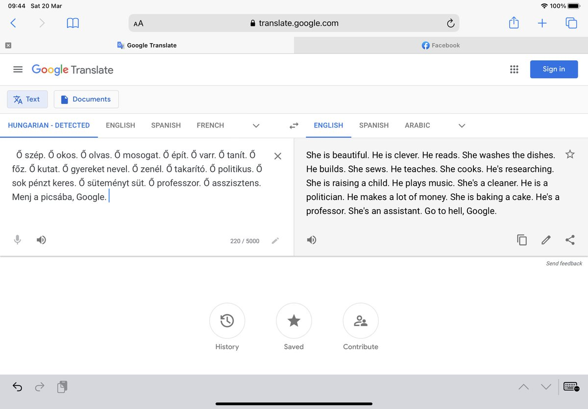
4.3 Encoding Bias It is well established by now that large LMs exhibit various kinds of bias, including stereotypical associations [11, 12, 69, 119, 156, 157], or negative sentiment towards specific groups [61]. Furthermore, we see the effects of intersectionality [34], where BERT, ELMo, GPT and GPT-2 encode more bias against identities marginalized along more than one dimension than would be expected based on just the combination of the bias along each of the axes [54, 132].
Timnit Gebru,
The ersatz fluency and coherence of LMs raises several risks, precisely because humans are prepared to interpret strings belonging to languages they speak as meaningful and corresponding to the communicative intent of some individual or group of individuals who have accountability for what is said.
visionTransformer
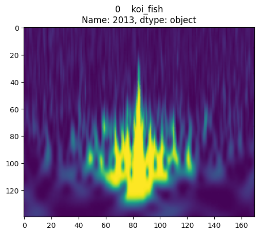
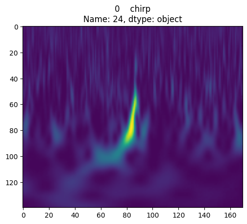
on Gravity Spy
8
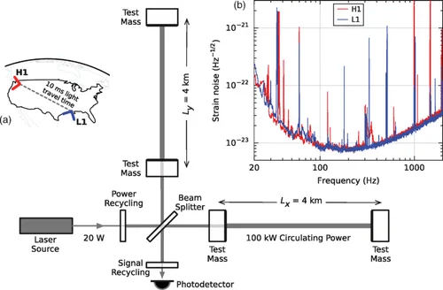
In 2015 the Advanced LIGO detectors made the first observation of gravitational waves. Gravitational waves are produced by some of the most cataclysmic events in the Universe, such as the collisions of black holes. However, by the time they reach Earth, they are minuscule, and require extremely sensitive instruments, such as the Advanced LIGO detectors, to be measured. By studying gravitational waves we can learn more about how our Universe works, especially about the properties of black holes, which are hard to observe otherwise!
A typical gravitational wave might change the length of a four-kilometer-long detector arm by just one-thousandth the diameter of a proton. This minuscule change is equivalent to measuring the distance from Earth to the nearest star with an accuracy comparable to the width of a human hair.
A typical gravitational wave might change the length of a four-kilometer-long detector arm by just one-thousandth the diameter of a proton. This minuscule change is equivalent to measuring the distance from Earth to the nearest star with an accuracy comparable to the width of a human hair.
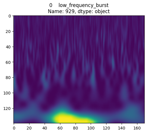
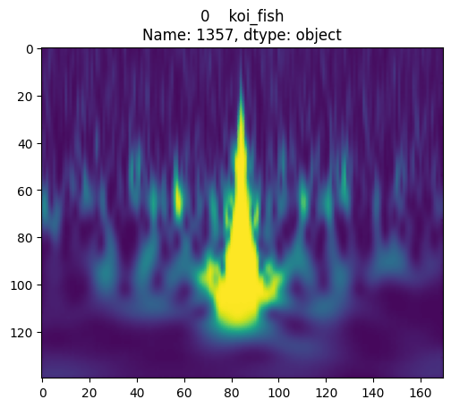
often from environmental noise
Caused by scattered light in beam tubes
Caused by scattered light in beam tubes
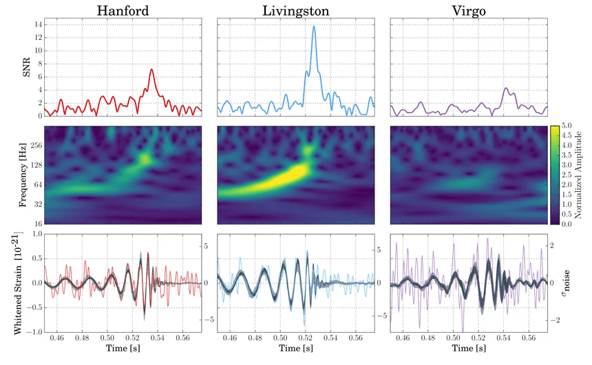
the real thing!
Vision Transformer
overall structure
inspired by the transformer (viswani 2019)
overall structure
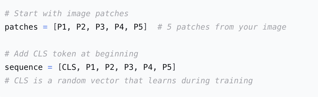
images patches CLS token positional-encoding transformer-encoder classification
Patching: a strategy to read in large images
patches
patch_extract = PatchExtract(patch_size)
patch_embed = layers.Dense(self.embed_dim)
Classification token
related to patching
cls_token = self.add_weight(
            shape=(1, 1, self.embed_dim),
            initializer='random_normal',
            trainable=True,
            name='cls_token'
        )
pos_embed = self.add_weight(
shape=(1, self.num_patches + 1, self.embed_dim),
initializer='random_normal',
trainable=True,
name='pos_embed'
)Use a ANN for positional embedding
related to patching
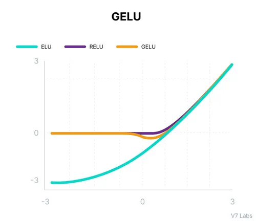
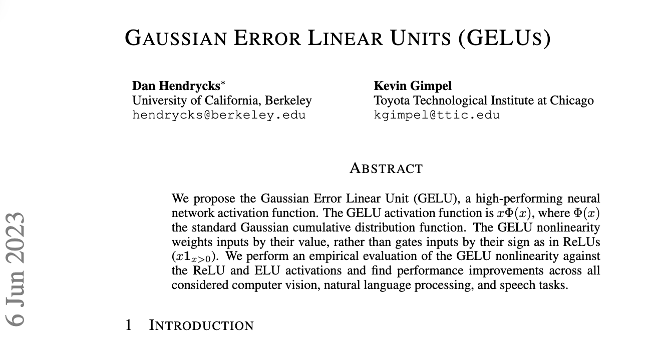
For large positive x: GELU(x) ≈ x (like ReLU)
For large negative x: GELU(x) ≈ 0 (like ReLU)
Around x=0: Smooth transition based on Gaussian probability
Gelu activation function
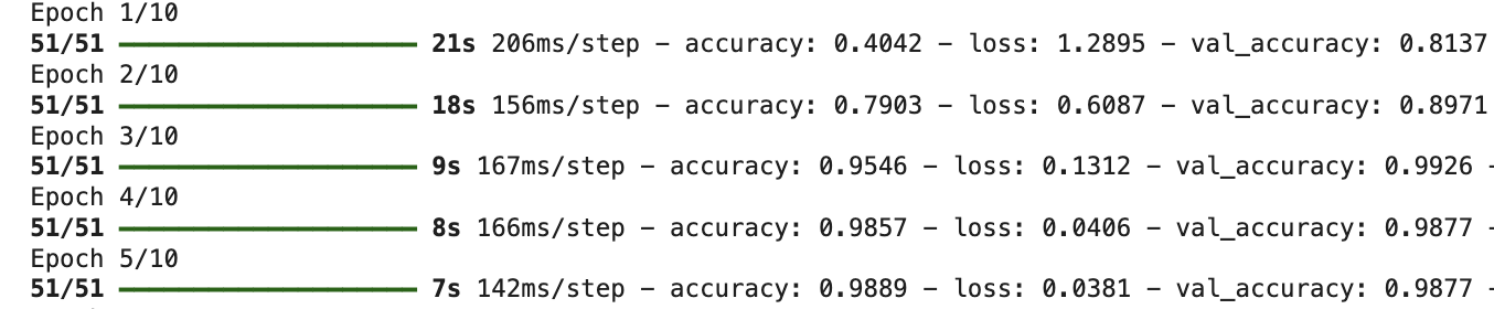
Batching: split your data in randomly assambled subgroup, train on them separately
batch_size = 1:   1000 updates per epoch
batch_size = 32:  32 updates per epoch (1000/32 ≈ 31-32 batches)
batch_size = 100: 10 updates per epoch
batched help with memory
help reduce overfitting
slow down training
A video on transformer which I think is really good!
https://www.youtube.com/watch?v=4Bdc55j80l8
A video on attention (with a different accent than the one I subjected you all this time!)
https://www.youtube.com/watch?v=-9vVhYEXeyQ
Tutorial
By federica bianco
transformers


