


federica bianco PRO
astro | data science | data for good
dr.federica bianco | fbb.space | fedhere | fedhere
IV: Machine Learning & Linear Regression
what is machine learning?
1
a model is a low dimensional representation of a higher dimensionality datase
the best way to think about it in the ML context:
what is a model?
[Machine Learning is the] field of study that gives computers the ability to learn without being explicitly programmed.
Arthur Samuel, 1959
model
parameters: slope, intercept
[Machine Learning is the] field of study that gives computers the ability to learn without being explicitly programmed.
Arthur Samuel, 1959
[Machine Learning is the] field of study that gives computers the ability to learn without being explicitly programmed.
Arthur Samuel, 1959
model
parameters: slope, intercept
data
ML: any model with parameters learnt from the data
ML: any model with parameters learnt from the data
Machine Learning models are parametrized representation of "reality" where the parameters are learned from finite sets (the sample) of realizations of that reality (the population)
(note: learning by instance, e.g. nearest neighbours, may not comply to this definition)
Machine Learning is the disciplines that conceptualizes, studies, and applies those models.
Key Concept
what is machine learning?
used to:
unsupervised vs supervised learning
Clustering
partitioning the feature space so that the existing data is grouped (according to some target function!)
understand the structure of a feature space
Clustering
partitioning the feature space so that the existing data is grouped (according to some target function!)
Unsupervised learning
All features are observed for all datapoints
unsupervised vs supervised learning
understand the structure of a feature space
Clustering
partitioning the feature space so that the existing data is grouped (according to some target function!)
Classifying & regression
finding functions of the variables that allow to predict unobserved properties of new observations
Unsupervised learning
All features are observed for all datapoints
unsupervised vs supervised learning
prediction and classification based on examples
Clustering
partitioning the feature space so that the existing data is grouped (according to some target function!)
Classifying & regression
finding functions of the variables that allow to predict unobserved properties of new observations
Unsupervised learning
Supervised learning
All features are observed for all datapoints
Some features are not observed for some data points we want to predict them.
unsupervised vs supervised learning
prediction and classification based on examples
Unsupervised learning
Supervised learning
All features are observed for all datapoints
and we are looking for structure in the feature space
Some features are not observed for some data points we want to predict them.
The datapoints for which the target feature is observed are said to be "labeled"
Semi-supervised learning
Active learning
A small amount of labeled data is available. Data is cluster and clusters inherit labels
The code can interact with the user to update labels and update model.
also...
unsupervised vs supervised learning
extract features and create models that allow prediction where the correct answer is known for a subset of the data
supervised learning
identify features and create models that allow to understand structure in the data
unsupervised learning
k-Nearest Neighbors
Regression
Support Vector Machines
Classification/Regression Trees
Neural networks
clustering
Principle Component Analsysis
Apriori (association rule)
what is a model?
2
line model:
y = ax+b
A model is a mathematical formula that represents (a simplified version of) a phenomenon.
Models have:
dependent/endogenous variables : y
A model is a mathematical formula that represents (a simplified version of) a phenomenon.
Models have:
dependent/endogenous variables : y
independent/exogenous variables : x
line model:
y = ax+b
~ x
A model is a mathematical formula that represents (a simplified version of) a phenomenon.
Models have:
dependent/endogenous variables : y
independent/exogenous variables : x
parameters : e.g. slope and intercept of a line which will be chosen based on the data
line model:
y = ax+b
A model is a mathematical formula that represents (a simplified version of) a phenomenon.
Models have:
dependent/endogenous variables : y
independent/exogenous variables : x
parameters : e.g. slope and intercept of a line which will be chosen based on the data
hyperparameters : all choices about a model that I will have to make that will not be directed by the data
line model:
y = ax+b
1
choose your model :
choose a mathematical formula to represent the behavior you see/expect in the data
line model: ax+b
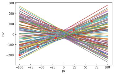
but there exist inifinite lines corresponding to infinite values of of slope and intercept
1
choose your model :
choose a mathematical formula to represent the behavior you see/expect in the data
line model: ax+b
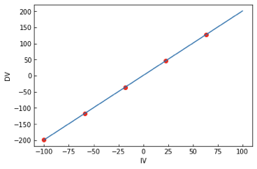
a mathematical formula describes a family of shapes. The parameters define the exact shape: in a line fit the parameters are...
- a: slope
- b: intercept
but there exist inifinite lines corresponding to infinite values of of slope and intercept
1
choose your model :
choose a mathematical formula to represent the behavior you see/expect in the data
polynomial model:
generalizatoin to a polynomial fit:
- the degree N of the polynomial is a hyperparameter of the model
we choose hyperparameters,
we fit parameters
N=12: goes exactly through each data point but it has too many parameters- N = number of data points
N=2: a conservative hyperparameter choice
1
choose your model :
choose a mathematical formula to represent the behavior you see/expect in the data
polynomial model:
generalizatoin to a polynomial fit:
- the degree N of the polynomial is a hyperparameter of the model
we choose hyperparameters,
we fit parameters
N=2: a conservative hyperparameter choice
2
choose an objective function :
you need a plan to choose the parameters of the model: to "optimize" the model.
You need to choose something to be MINIMIZED or MAXIMIZED
line model: ax+b
but there exist inifinite lines corresponding to infinite values of of slope and intercept
In principle, there are many choices for objective function. But the only procedure that is truly justified—in the sense that it leads to interpretable probabilistic inference, is to make a generative model for the data.
what you want to optimize for
what you want to optimize for
what you want to optimize for
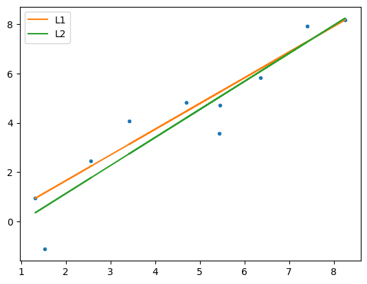
L1 or Sum of Absolute Errors:
what you want to optimize for
L1 or Sum of Absolute Errors:
model prediction
what you want to optimize for
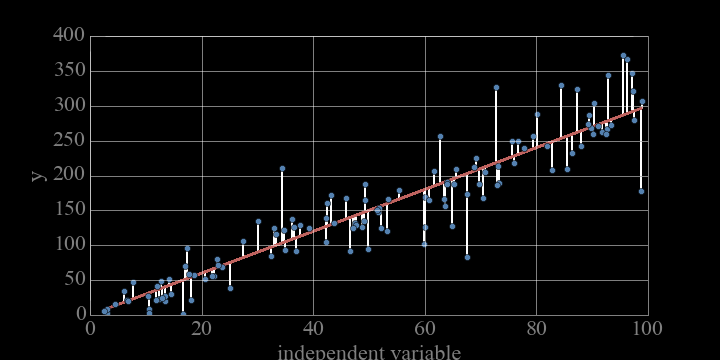
L2 or Sum of Squared Errors:
what you want to optimize for
Fit model parameters <==> minimize the objective function
yi: i-th observation
xi: i-th measurement "location"
NOTE: Sum of residual squared (least square fit method)
what you want to optimize for
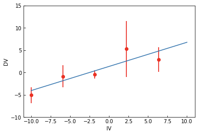
Same data, same model, different solution!
WHY???
2
choose an objective function :
you need a plan to choose the parameters of the model: to "optimize" the model.
You need to choose something to be MINIMIZED or MAXIMIZED
line model: ax+b
a line is a family of models
a line with set parameters is a models
why do we model?
2.1
why do we model?
to explain
to predict
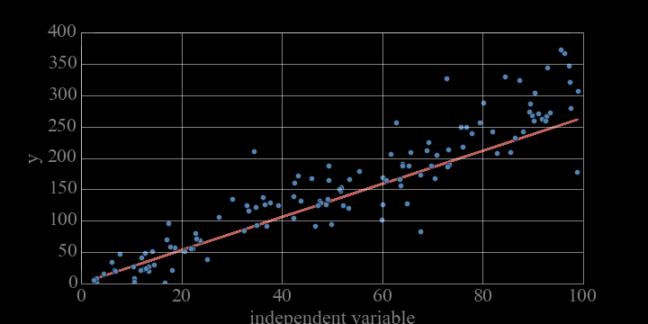
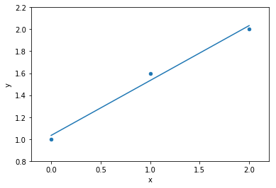
fitting a line to data
(the longish story)
3
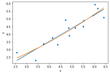
We are trying to find the "best" line that goes through the data... but "best" is a judgment call
We are trying to find the "best" line that goes through the data... but "best" is a judgment call
Choosing the objective function
We are trying to find the "best" line that goes through the data... but "best" is a judgment call
minimize something:
minimize something:
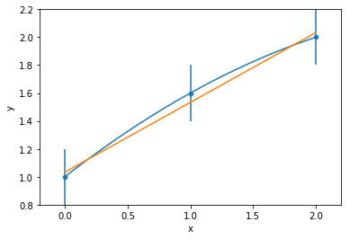
why square?
- So that the errors do not cancel themselves out
- To add more weight to predictions that are worse
Ordinary least square
minimize something:
def sumsqerror(y, yp):
  ''' objective function squared error
  y: vector of observations
  yp: vector of predictions
  return: sum squared difference
  '''
  return ((y - yp) ** 2).sum()

minnow = 1e7
for s in np.arange(0, 3, 0.01):
  for i in np.arange(0, 2.5, 0.01):
    prediction = df['population'] * s + i
    sse = sumsqerror(df.wspeed, prediction)
    if sse < minnow:
      minnow = sse
      slope_manual, inrercept_manual = s, i

slope_manual, inrercept_manual
we can minimize manually...
Ordinary least square
We are trying to find the "best" line that goes through the data... but "best" is a judgment call
minimize something:
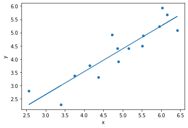
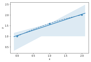
but its a lot easier to use
built in functions
# seaborn (just plots)
sns.regplot(df['population'], df['wspeed'])
# numpy
slope, intercept = np.polyfit(df['population'], df['wspeed'], 1)
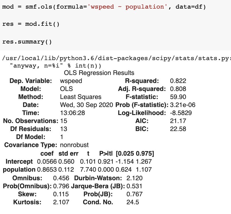
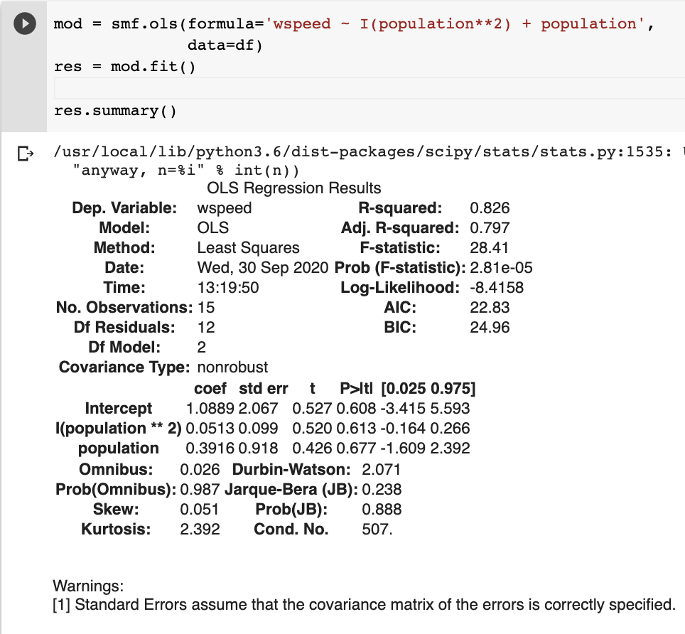
# statsmodels formula
smf.ols(formula='wspeed ~ population', data=df)
# statsmodels OLS works for any degree polynomial
polynomial_features = PolynomialFeatures(degree=1)
xp1 = polynomial_features.fit_transform(x)
model = sm.OLS(y[:10], xp1[:10]).fit()
We are trying to find the "best" line that goes through the data... but "best" is a judgment call
minimize something:
but its a lot easier to use
built in functions
# seaborn (just plots)
import seaborn as sns
sns.regplot(df['population'], df['wspeed'])

# numpy
import numpy as np
slope, intercept = np.polyfit(df['population'], df['wspeed'], 1)

# statsmodels formula
import statsmodels.formula.api as smf
smf.ols(formula='wspeed ~ population', data=df)

# statsmodels OLS works for any degree polynomial
from sklearn.preprocessing import PolynomialFeatures
polynomial_features = PolynomialFeatures(degree=1)
xp1 = polynomial_features.fit_transform(x)
model = sm.OLS(y[:10], xp1[:10]).fit()

# sklearn
from sklearn.linear_model import LinearRegression
lm = LinearRegression().fit(X_train, y_train, sample_weight=None)
how good is the model?
but its a lot easier to use
built in functions
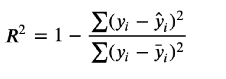
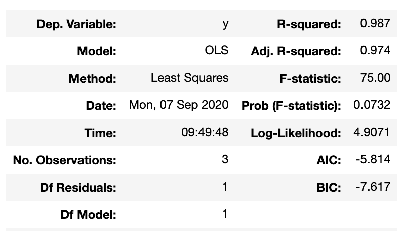
SSE ( prediction)
variance ( mean)
but its a lot easier to use
built in functions
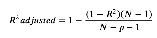
Adjusted R2 takes into account how many datapoints you have and how many paramters you have
how good is the model?
but its a lot easier to use
built in functions
- increasing the model complexity increases the R2 but does not guarantee a better model
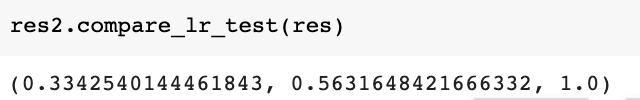
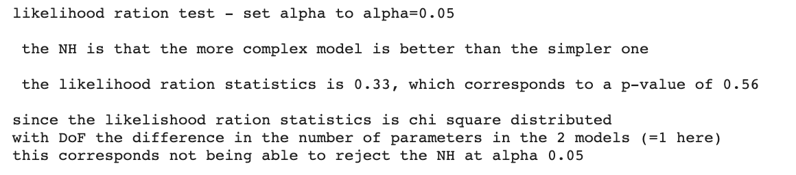
- the likelihood ratio is a way to assess if the more complex model is better in a NHRT sense
but its a lot easier to use
built in functions
- increasing the model complexity increases the R2 but does not guarantee a better model
- the likelihood ratio is a way to assess if the more complex model is better in a NHRT sense
NH: the more complex model is better
under the NH the LR statistics is distributed like a chi^2 distribution with number of dof = number of extra parameters
p-value of LR in a chi^2 distribution with dof
but its a lot easier to use
built in functions
- increasing the model complexity increases the R2 but does not guarantee a better model
- the likelihood ratio is a way to assess if the more complex model is better in a NHRT sense
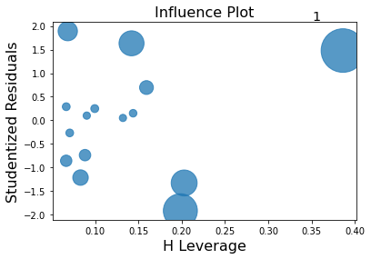
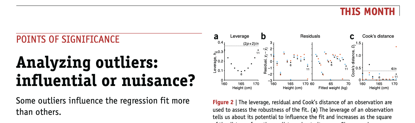
not all points are equal!
This function creates a “bubble” plot of Studentized residuals versus hat leverage values.
hi residual: outlier on the Y axis
high leverage : at the edge of the X axis
influence analysis
identify data points that have strong influence on the model fit: unusual x values or their y value is an "outlier". Points that are both are on the top right of the plot and are high influence points. Cook's distance is represented by the size of the bubble.
It can be shown that OLS minimization of the sum of the square errors (SSE) is equivalent to calculating the slope and intercept as:
Normal equation
how do we model?
Choose the model:
a mathematical formula to represent the behavior in the data
1
example: line model y = a x + b
parameters
how do we model?
Choose the model:
a mathematical formula to represent the behavior in the data
1
example: line model y = a x + b
parameters
Choose the hyperparameters:
parameters chosen before the learning process, which govern the model and training process
example: the degree N of the polynomial
how do we model?
Choose an objective function:
in order to find the "best" parameters of the model: we need to "optimize" a function.
We need something to be either MINIMIZED or MAXIMIZED
2
example:
line model: y = a x + b
parameters
objective function: sum of residual squared (least square fit method)
we want to minimize SSE as much as possible
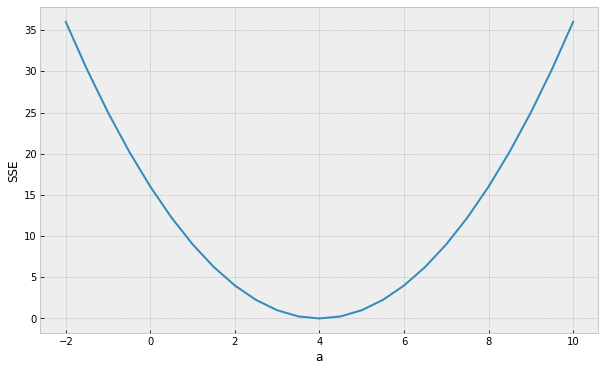
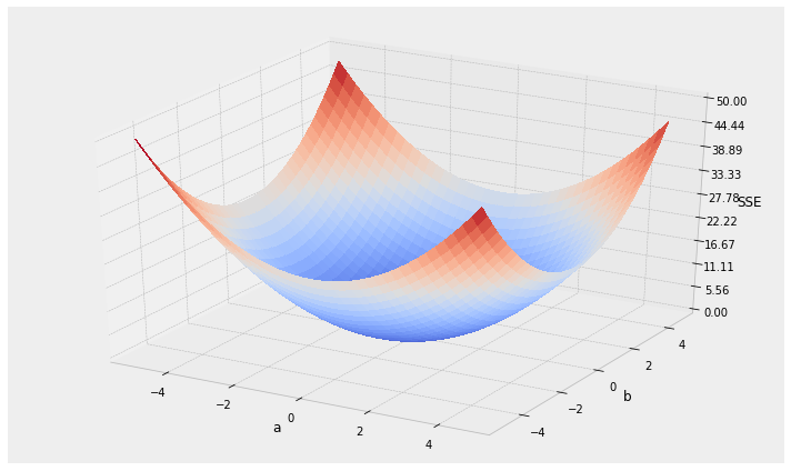
Optimizing the Objective Function
assume a simpler line model y = ax
(b = 0) so we only need to find the "best" parameter a
assume a simpler line model y = ax
(b = 0) so we only need to find the "best" parameter a
Minimum (optimal) SSE
a = 4
Optimizing the Objective Function
assume a simpler line model y = ax
(b = 0) so we only need to find the "best" parameter a
How do we find the minimum if we do not know beforehand how the SSE curve looks like?
Optimizing the Objective Function
Minimum (optimal) SSE
a = 4
3.1
stochastic gradient descent (SGD)
what is a machine learning?
1
2
3
4
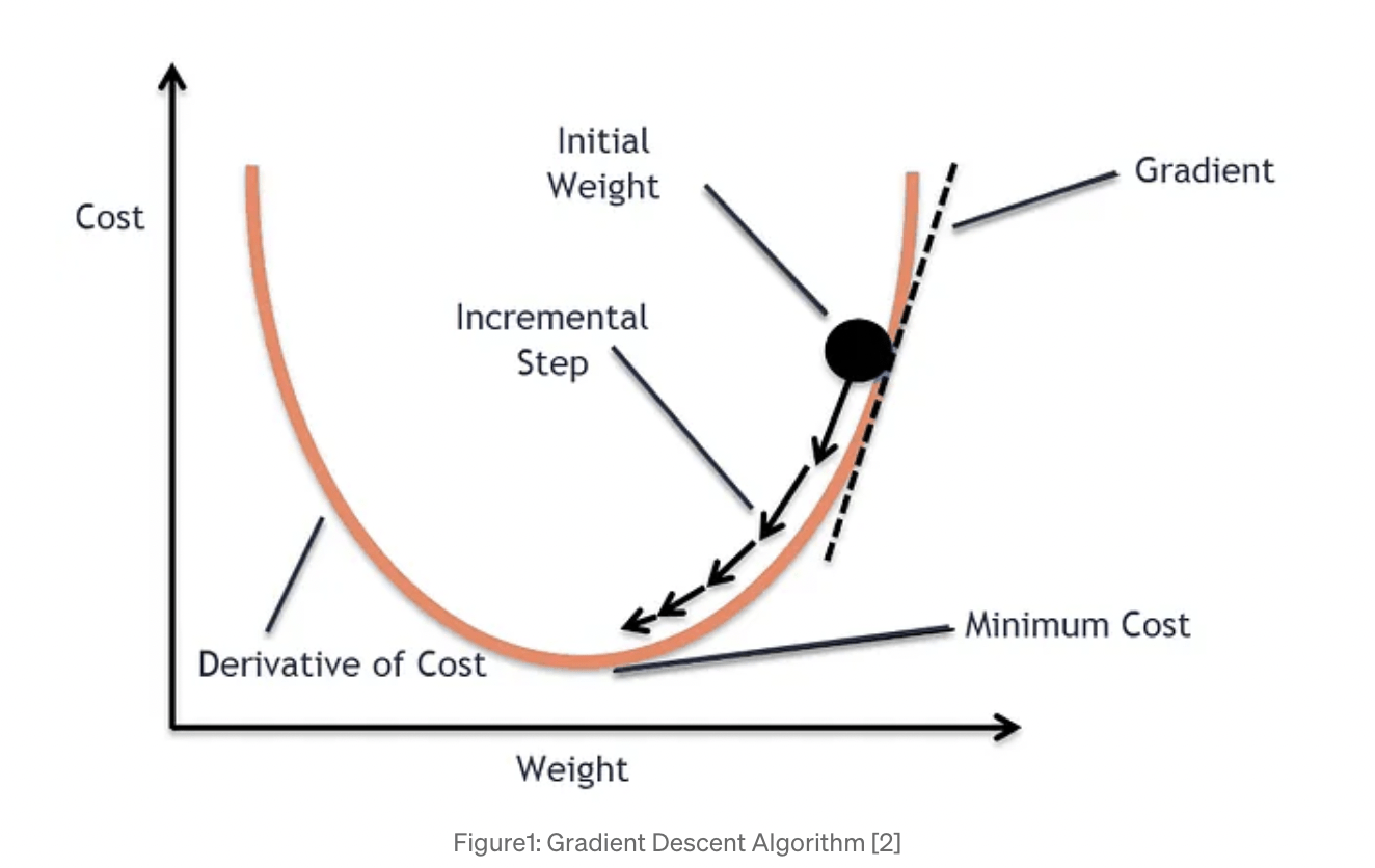
the algorithm: Stochastic Gradient Descent (SGD)
assume a simpler line model y = ax
(b = 0) so we only need to find the "best" parameter a
the algorithm: Stochastic Gradient Descent
assume a simpler line model y = ax
(b = 0) so we only need to find the "best" parameter a
1. choose initial value for a
-1
the algorithm: Stochastic Gradient Descent
assume a simpler line model y = ax
(b = 0) so we only need to find the "best" parameter a
1. choose initial value for a=a0
2. calculate the loss at a0 : SSE(a0)
the algorithm: Stochastic Gradient Descent
assume a simpler line model y = ax
(b = 0) so we only need to find the "best" parameter a
1. choose initial value for a=a0
2. calculate the loss at a0 : SSE(a0)
3. calculate best direction to go to decrease the SSE
the algorithm: Stochastic Gradient Descent
assume a simpler line model y = ax
(b = 0) so we only need to find the "best" parameter a
1. choose initial value for a=a0
2. calculate the loss at a0 : SSE(a0)
3. calculate best direction to go to decrease the SSE
the algorithm: Stochastic Gradient Descent
assume a simpler line model y = ax
(b = 0) so we only need to find the "best" parameter a
1. choose initial value for a=a0
2. calculate the loss at a0 : SSE(a0)
3. calculate best direction to go to decrease the SSE
the algorithm: Stochastic Gradient Descent
assume a simpler line model y = ax
(b = 0) so we only need to find the "best" parameter a
1. choose initial value for a=a0
2. calculate the loss at a0 : SSE(a0)
3. calculate best direction to go to decrease the SSE
4. step in that direction
the algorithm: Stochastic Gradient Descent
assume a simpler line model y = ax
(b = 0) so we only need to find the "best" parameter a
1. choose initial value for a=a0
2. calculate the loss at a0 : SSE(a0)
3. calculate best direction to go to decrease the SSE
4. step in that direction
5. go back to step 2 and repeat
the algorithm: Stochastic Gradient Descent
for a line model y = ax + b
we need to find the "best" parameters a and b
1. choose initial value for a & b
2. calculate the SSE(a0,b0)
3. calculate best direction to go to decrease the SSE
4. step in that direction
5. go back to step 2 and repeat
the algorithm: Stochastic Gradient Descent
for a line model y = ax + b
we need to find the "best" parameters a and b
1. choose initial value for a & b
2. calculate the SSE(a0,b0)
3. calculate best direction to go to decrease the SSE
4. step in that direction
5. go back to step 2 and repeat
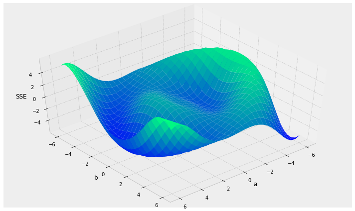
the algorithm: Stochastic Gradient Descent
Things to consider:
the algorithm: Stochastic Gradient Descent
Things to consider:
- local vs. global minima
local minima
global minimum
the algorithm: Stochastic Gradient Descent
Things to consider:
- local vs. global minima
- initialization: choosing starting spot?
global minimum
local minima
the algorithm: Stochastic Gradient Descent
Things to consider:
- local vs. global minima
Stochastic Gradient Descent (SGD): use a different (random) sub-sample of the data at each iteration
also: try different starting points and do multiple minimization (computationally expensive)
also: sometimes also go uphill (MonteCarlo methods)
the algorithm: Stochastic Gradient Descent
Things to consider:
- local vs. global minima
- initialization: choosing starting spot?
- learning rate: how far to step?
the algorithm: Stochastic Gradient Descent
Things to consider:
- local vs. global minima
- initialization: choosing starting spot?
- learning rate: how far to step?
the algorithm: Stochastic Gradient Descent
Things to consider:
- local vs. global minima
- initialization: choosing starting spot?
- learning rate: how far to step?
the algorithm: Stochastic Gradient Descent
Things to consider:
- local vs. global minima
- initialization: choosing starting spot?
- learning rate: how far to step?
the algorithm: Stochastic Gradient Descent
Things to consider:
- local vs. global minima
- initialization: choosing starting spot?
- learning rate: how far to step?
the algorithm: Stochastic Gradient Descent
assume a simpler line model y = ax
(b = 0) so we only need to find the "best" parameter a
1. choose initial value for a
2. calculate the SSE
3. take the gradient of the SSE and step in proportion
: the gradient is the slope of a line tangential to a point on a curve
the algorithm: Stochastic Gradient Descent
Things to consider:
- local vs. global minima
- initialization: choosing starting spot?
- learning rate: how far to step?
Adaptive learning rate: fast early on, slow later. Very common with Neural Networks
the algorithm: Stochastic Gradient Descent
Things to consider:
- local vs. global minima
- initialization: choosing starting spot?
- learning rate: how far to step?
- stopping criterion: when to stop?
epistemological rooots of overfitting
4
overfitting
Ockham’s razor: Pluralitas non est ponenda sine neccesitate
or “the law of parsimony”
William of Ockham (logician and Franciscan friar) 1300ca
but probably to be attributed to John Duns Scotus (1265–1308)
”Complexity needs not to be postulated without a need for it”
“Between 2 theories choose the simpler one”
“Between 2 theories choose the one with fewer parameters"
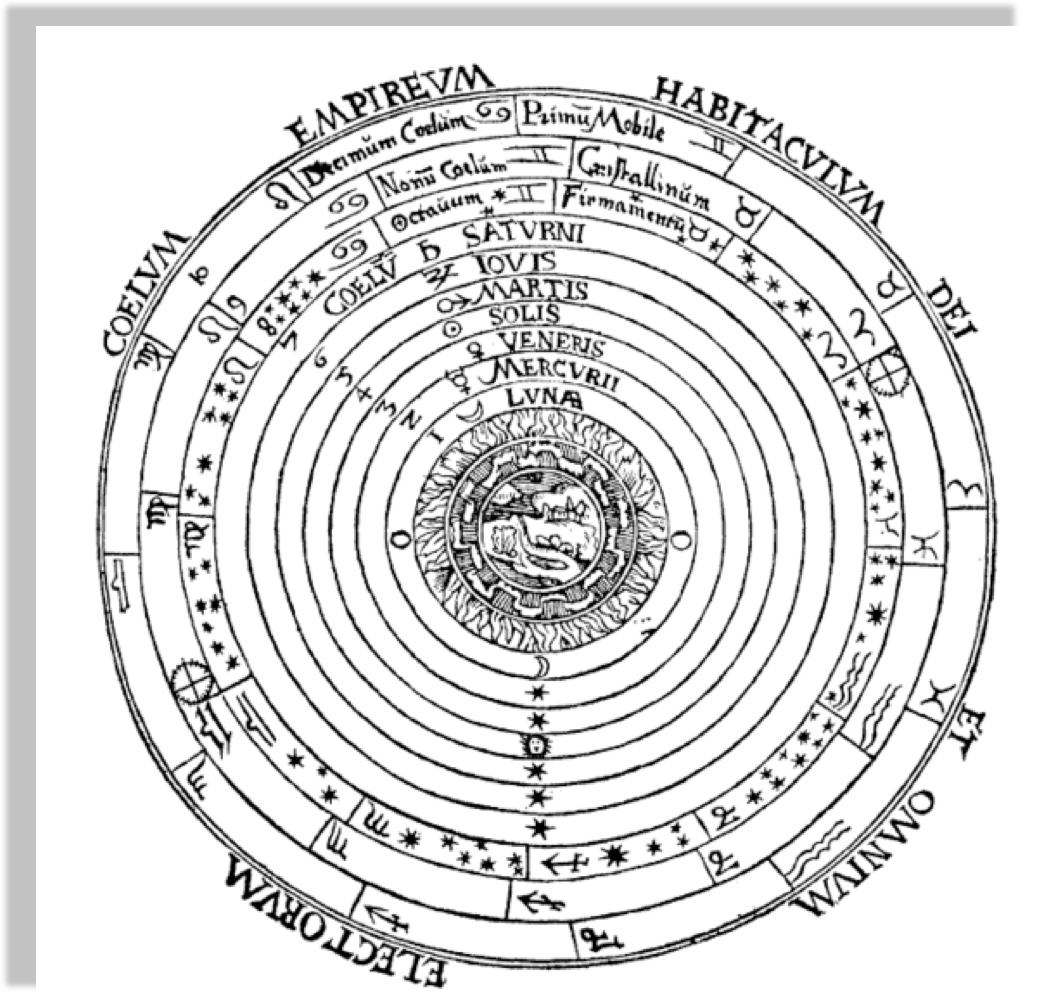
From the Greeks to Peter Apian, Cosmographia, Antwerp, 1524
Author Dr Long's copy of Cassini, 1777
From the Greeks to Peter Apian, Cosmographia, Antwerp, 1524
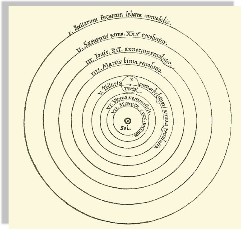
Heliocentric model from Nicolaus Copernicus'
"De revolutionibus orbium coelestium".
Author Dr Long's copy of Cassini, 1777
From the Greeks to Peter Apian, Cosmographia, Antwerp, 1524
Heliocentric model from Nicolaus Copernicus'
"De revolutionibus orbium coelestium".
Author Dr Long's copy of Cassini, 1777
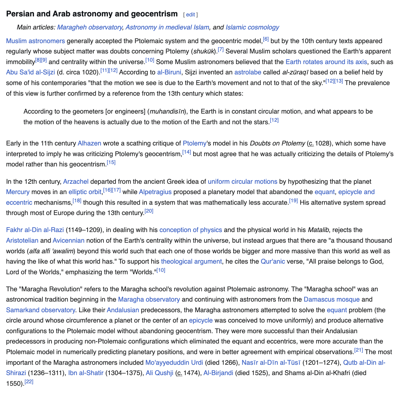
Two theories may explain a phenomenon just as well as each other. In that case you should prefer the simpler one
Meanwhile, in the Arab world geocentrism was being questioned as early as the IX century
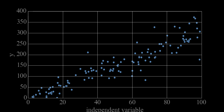
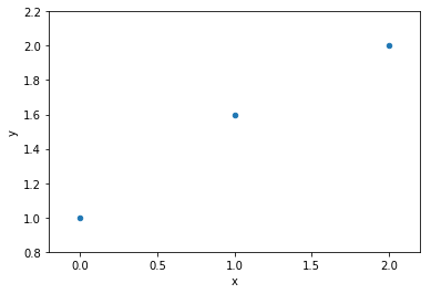
data
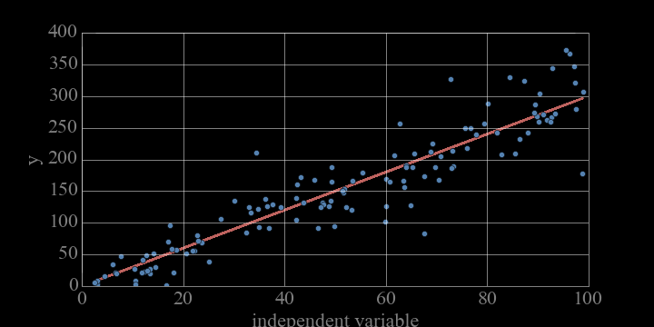
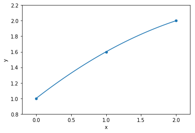
model fit to data
model fit to data
model fit to data
1 variable: x
model fit to data
parameters
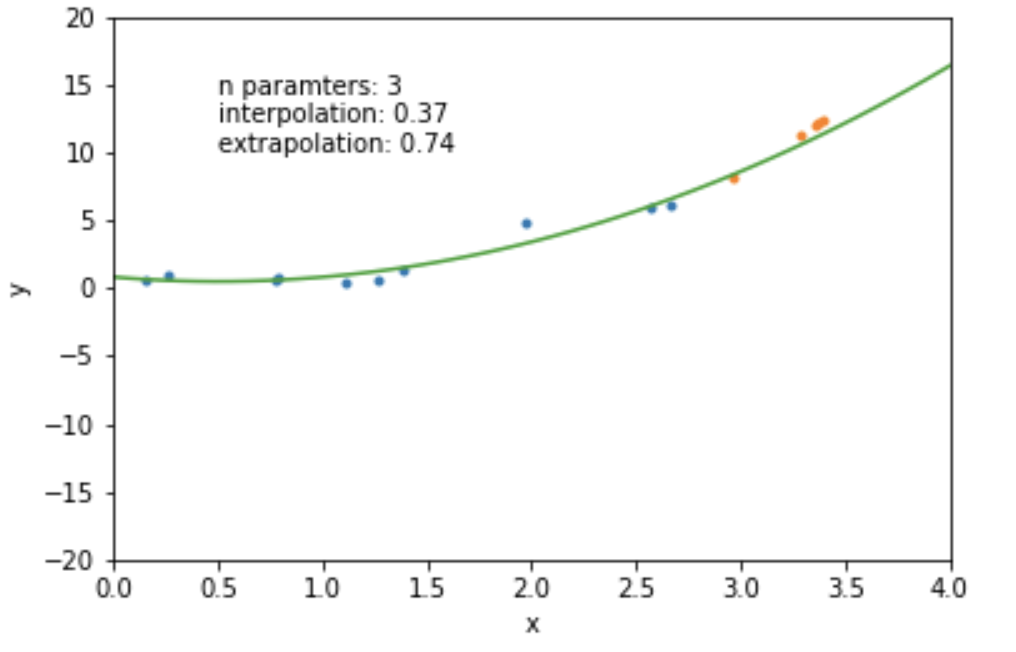
the complexity of a model can be measured by the number of variables and the numbers of parameters
the complexity of a model can be measured by the number of variables and the numbers of parameters
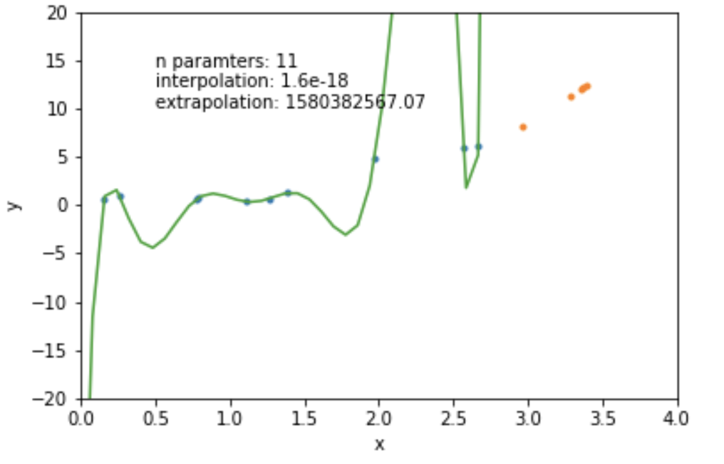
mathematically: given N data points there exist an N-features model that goes exactly through each data point. but is it useul??
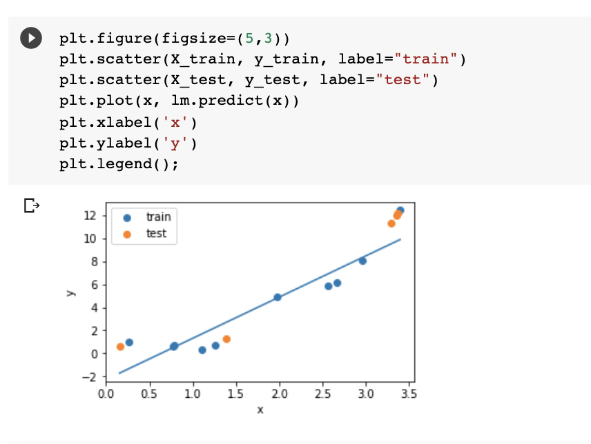
Overfitting: fitting data with a model that is too complex and that does not extend to new data (low predictive power on test data)
data
model fit to data
how to avoid overfitting in machine learning
5
overfitting
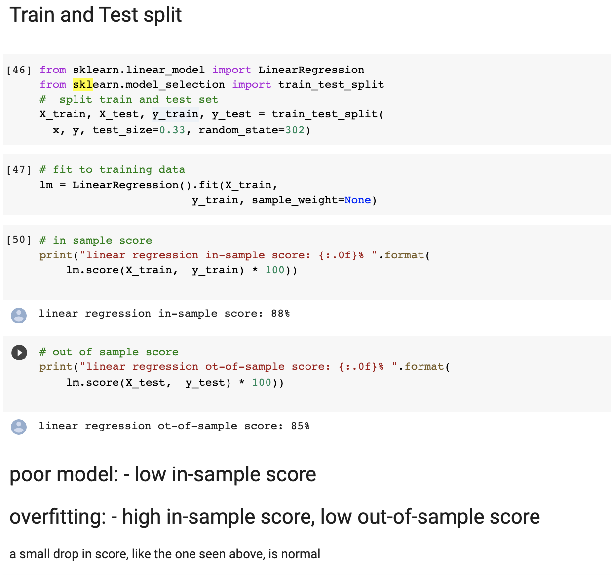
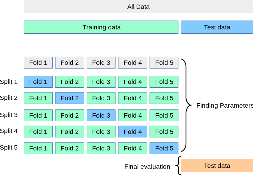
test train validation
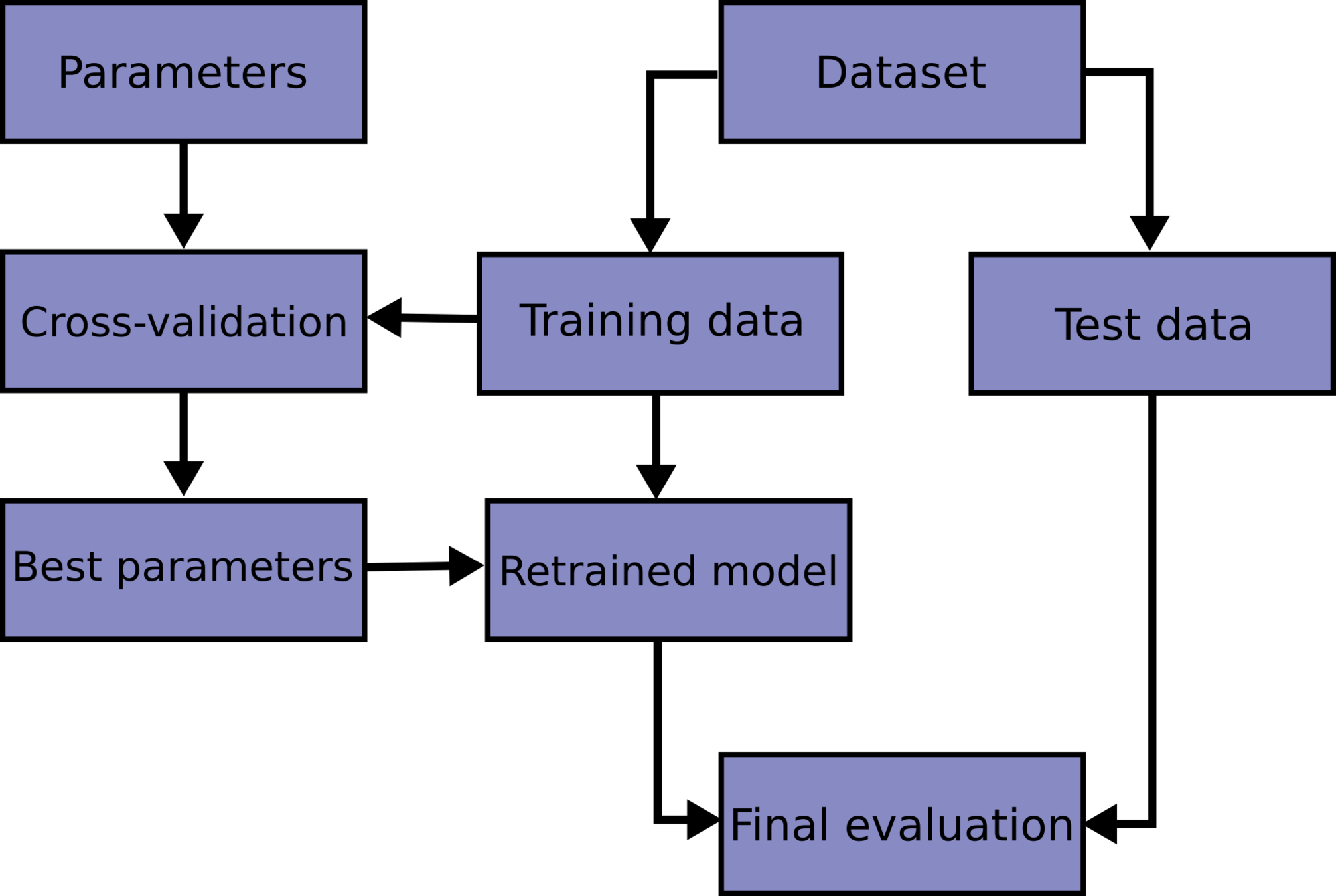
train parameters on training set
run only once on the test set to assess the model performance
test + train + validation
train parameters on training set
adjust parameters on validation set
run only once on the test set to assess the model performance
k-fold cross validation
10/4 MIDTERM
10/4 : MIDTERM in class
what is covered in the midterm? everything we do until 9/31!
how is the midterm graded?
RULES: work on your on, ALL CAMERAS MUST BE ON
The grading scheme reflects the complexity of the tasks and the expectation of how well they have been absorbed based on how long we have been working on it
line models and polynomial models
parameters and hyperparameters
objective function: what do we minimize to choose parameters?
model diagnostics and choosing models
influence points
cross validation
this is a pretty comprehensive and clear medium post with coding examples
this is a whole paper about modeling in practice and in theory which covers extensively how to deal with uncertainties. it is not for the faint of heart. The notes are entertaining
By federica bianco
Machine Learning and linear regression


