federica bianco PRO
astro | data science | data for good
VI: Logistic Regression
AUTHOR AND LECTURER: Farid Qamar
this slide deck: https://slides.com/faridqamar/fdfse_6
0
optimizing the objective function
what is a model?
in the ML context:
a model is a low dimensional representation of a higher dimensionality dataset
recall:
what is a machine learning?
ML: Any model with parameters learned from the data
what is a machine learning?
ML: Any model with parameters learned from the data
ML models are a parameterized representation of "reality" where the parameters are learned from finite sets (samples) of realizations of that reality (population)
how do we model?
Choose the model:
a mathematical formula to represent the behavior in the data
1
example: line model y = a x + b
parameters
how do we model?
Choose the model:
a mathematical formula to represent the behavior in the data
1
example: line model y = a x + b
parameters
Choose the hyperparameters:
parameters chosen before the learning process, which govern the model and training process
example: the degree N of the polynomial
how do we model?
Choose an objective function:
in order to find the "best" parameters of the model: we need to "optimize" a function.
We need something to be either MINIMIZED or MAXIMIZED
2
example:
line model: y = a x + b
parameters
objective function: sum of residual squared (least square fit method)
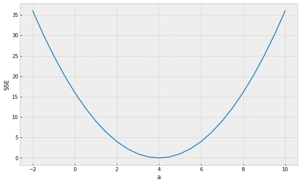
we want to minimize SSE as much as possible
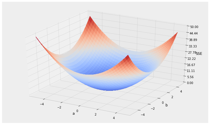
Optimizing the Objective Function
assume a simpler line model y = ax
(b = 0) so we only need to find the "best" parameter a
assume a simpler line model y = ax
(b = 0) so we only need to find the "best" parameter a
Minimum (optimal) SSE
a = 4
Optimizing the Objective Function
assume a simpler line model y = ax
(b = 0) so we only need to find the "best" parameter a
How do we find the minimum if we do not know beforehand how the SSE curve looks like?
Optimizing the Objective Function
Minimum (optimal) SSE
a = 4
1
multilinear regression
ML terminology
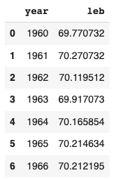
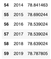
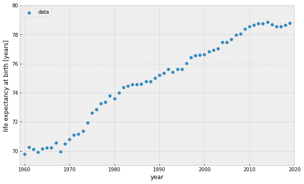
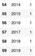
World Bank: Life expectancy at birth in the US
ML terminology
World Bank: Life expectancy at birth in the US
ML terminology
World Bank: Life expectancy at birth in the US
model
ML terminology
World Bank: Life expectancy at birth in the US
object
model
ML terminology
World Bank: Life expectancy at birth in the US
object
feature
model
ML terminology
World Bank: Life expectancy at birth in the US
object
feature
target
model
ML terminology
objects
features
target
ML terminology
features
target
objects
Simple Linear Regression
1 feature
1 target
2 parameters
Simple Linear Regression
1 feature
1 target
2 parameters
Simple Linear Regression
1 feature
1 target
2 parameters
Multiple Linear Regression
n features
1 target
Simple Linear Regression
1 feature
1 target
2 parameters
Multiple Linear Regression
n features
1 target
n+1 parameters
Simple Linear Regression
1 feature
1 target
2 parameters
Multiple Linear Regression
;
n features
1 target
n+1 parameters
2
regression vs classification
Regression example:
find the optimal parameters (slope/coefficients and intercept) of a linear model that best combine the features (independent variables) to describe the target (dependent variable)
Regression example:
find the optimal parameters (slope/coefficients and intercept) of a linear model that best combine the features (independent variables) to describe the target (dependent variable)
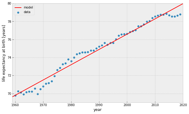
World Bank: Life expectancy at birth in the US
Regression example:
find the optimal parameters (slope/coefficients and intercept) of a linear model that best combine the features (independent variables) to describe the target (dependent variable)
World Bank: Life expectancy at birth in the US
target variable is continuous
Regression example:
find the optimal parameters (slope/coefficients and intercept) of a linear model that best combine the features (independent variables) to describe the target (dependent variable)
line model y = ax + b
Regression example:
find the optimal parameters (slope/coefficients and intercept) of a linear model that best combine the features (independent variables) to describe the target (dependent variable)
line model y = ax + b
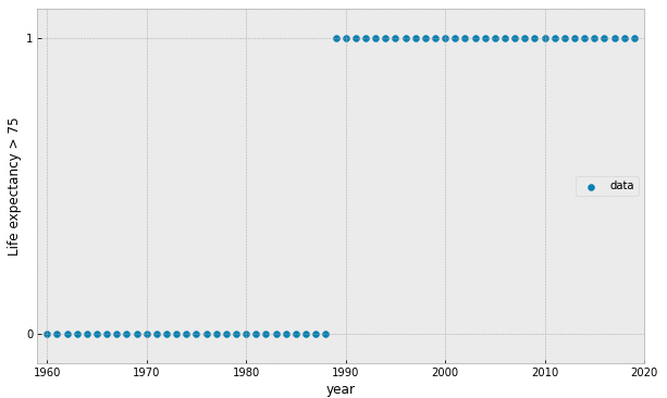
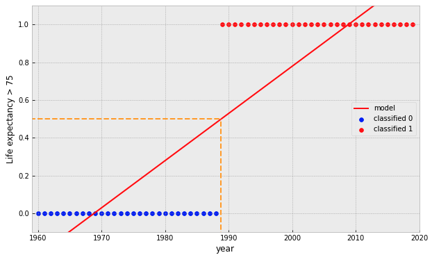
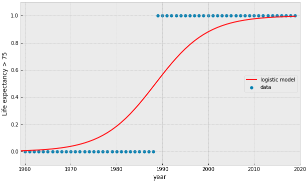
what if our data is represented by a binary value?
target variable is categorical
what if our data is represented by a binary value?
what if our data is represented by a binary value?
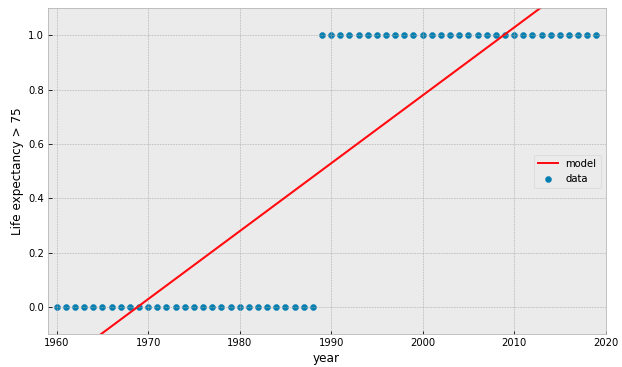
try fitting a linear model...
what if our data is represented by a binary value?
try fitting a linear model...
what if our data is represented by a binary value?
try fitting a linear model...
what if our data is represented by a binary value?
try fitting a linear model...
what if our data is represented by a binary value?
try fitting a linear model...
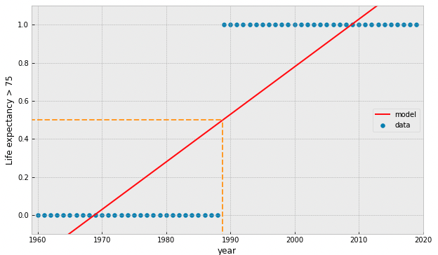
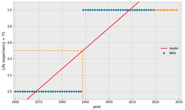
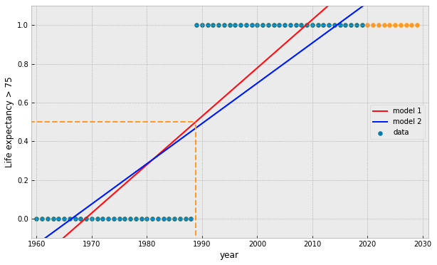
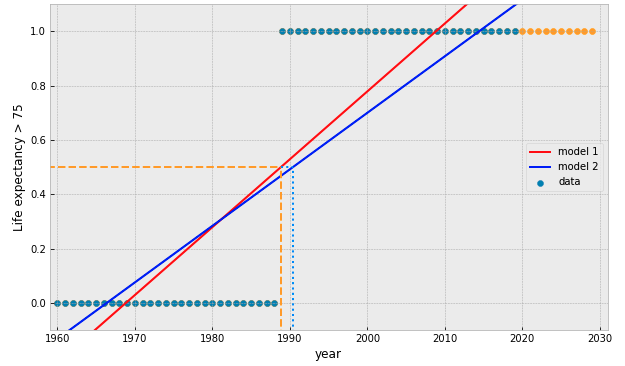
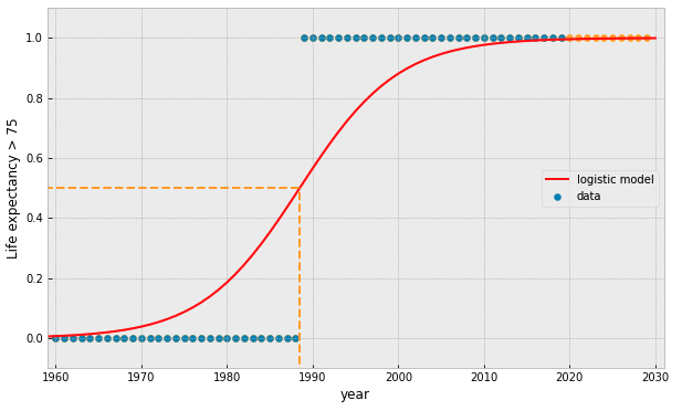
what if we add more data points?
what if our data is represented by a binary value?
try fitting a linear model...
what if we add more data points?
what if our data is represented by a binary value?
try fitting a linear model...
what if we add more data points?
3
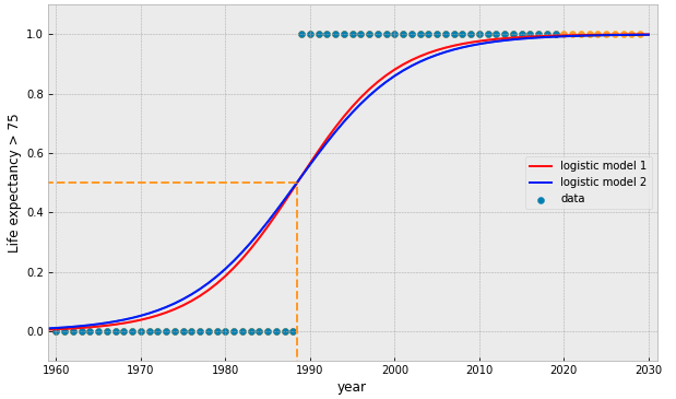
logistic regression
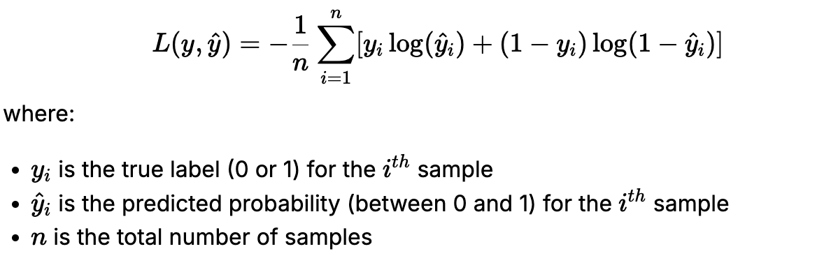
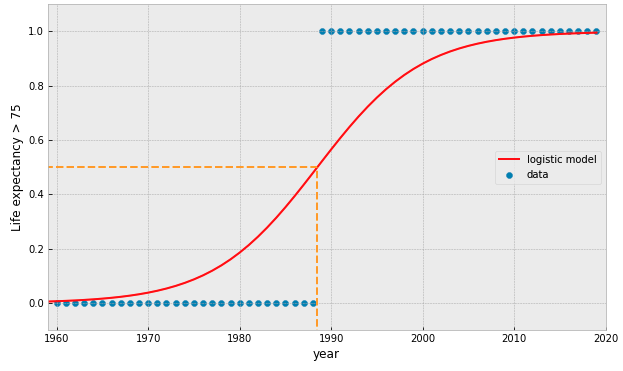
the Logistic Function:
interpreted as the probability that the target is True (= 1)
Objective Function:
Cross Entropy
the Logistic Function:
interpreted as the probability that the target is True (= 1)
Objective Function:
Cross Entropy
the Logistic Function:
interpreted as the probability that the target is True (= 1)
(Sigmoid)
Objective Function:
Cross Entropy
the Logistic Function:
interpreted as the probability that the target is True (= 1)
Objective Function:
Cross Entropy
the Logistic Function:
interpreted as the probability that the target is True (= 1)
what if we add more data points?
the Logistic Function:
interpreted as the probability that the target is True (= 1)
what if we add more data points?
4
classification model evaluation
indicates the model's "confusion" between classification outcomes
class 0
class 1
class 0
class 1
Predicted
Actual
smaller off-diagonal elements &
larger diagonal elements
=
model more effective at correctly labeling classes
indicates the model's "confusion" between classification outcomes
class 0
class 1
class 0
class 1
Predicted
Actual
smaller off-diagonal elements &
larger diagonal elements
=
model more effective at correctly labeling classes
class 2
class 2
indicates the model's "confusion" between classification outcomes
negative
positive
negative
positive
Predicted
Actual
smaller off-diagonal elements &
larger diagonal elements
=
model more effective at correctly labeling classes
for example...
model predicting 500 objects:
232
4
1
263
Predicted
Actual
232
4
1
263
TN
FP
TP
FN
negative
positive
negative
positive
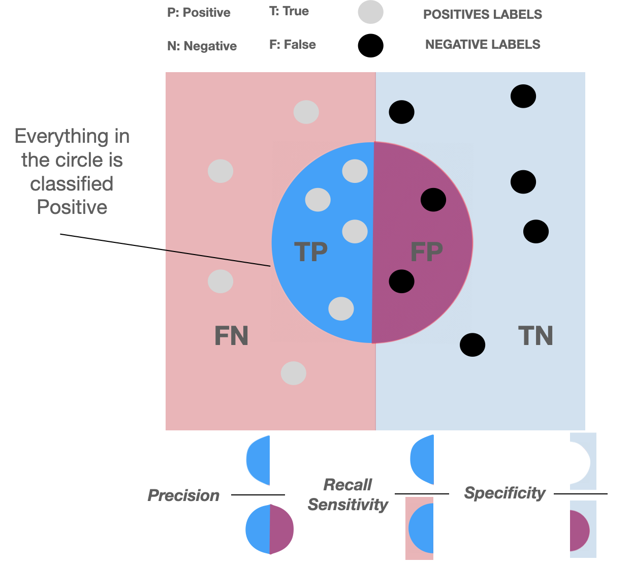
Classification outcomes:
true positives (TP) : "+" correctly labeled as "+"
true negatives (TN) : "-" correctly labeled as "-"
false positives (FP) : "-" incorrectly labeled as "+"
false negatives (FN) : "+" incorrectly labeled as "-"
Predicted
Actual
232
4
1
263
TN
FP
TP
FN
negative
positive
negative
positive
Classification outcomes:
true positives (TP) : "+" correctly labeled as "+"
true negatives (TN) : "-" correctly labeled as "-"
false positives (FP) : "-" incorrectly labeled as "+"
false negatives (FN) : "+" incorrectly labeled as "-"
accuracy:
accuracy =
Classification outcomes:
true positives (TP) : "+" correctly labeled as "+"
true negatives (TN) : "-" correctly labeled as "-"
false positives (FP) : "-" incorrectly labeled as "+"
false negatives (FN) : "+" incorrectly labeled as "-"
Predicted
Actual
232
4
1
263
TN
FP
TP
FN
negative
positive
negative
positive
precision:
recall:
precision =
recall =
precision:
(or specificity)
recall:
(or sensitivity)
Fraction of objects you think are positive that actually are positive
Fraction of positive objects that you were able to find
F1-score:
Current classifier accuracy: 50%
Precision?
Recall?
Specificity?
Sensitivity?
Current classifier accuracy: 50%
Precision = 4/6 = 0.7
Recall = 4/8 = 0.5
Specificity = 0.7
Sensitivity = 0.5
4
| spicies | age | weight |
|---|---|---|
| dog | 7 | 32.3 |
| bird | 1 | 0.3 |
| cat | 3 | 8.1 |
continuous
| spicies | age | weight |
|---|---|---|
| dog | 7 | 32.3 |
| bird | 1 | 0.3 |
| cat | 3 | 8.1 |
ordinal
| spicies | age | weight |
|---|---|---|
| dog | 7 | 32.3 |
| bird | 1 | 0.3 |
| cat | 3 | 8.1 |
continuous
categorical
ordinal
| spicies | age | weight |
|---|---|---|
| dog | 7 | 32.3 |
| bird | 1 | 0.3 |
| cat | 3 | 8.1 |
continuous
change categorical to (integer) numerical
| spicies | age | weight |
|---|---|---|
| 1 | 7 | 32.3 |
| 2 | 1 | 0.3 |
| 3 | 3 | 8.1 |
change each category to a binary
| cat | bird | dog | age | weight |
|---|---|---|---|---|
| 0 | 0 | 1 | 7 | 32.3 |
| 0 | 1 | 0 | 1 | 0.3 |
| 1 | 0 | 0 | 3 | 8.1 |
implies an order that does not exist
change categorical to (integer) numerical
| spicies | age | weight |
|---|---|---|
| 1 | 7 | 32.3 |
| 2 | 1 | 0.3 |
| 3 | 3 | 8.1 |
dog=1, bird=2, cat=3
...dog < bird < cat... ??
ignores covariance between features
increases the dimensionality
change each category to a binary
| cat | bird | dog | age | weight |
|---|---|---|---|---|
| 0 | 0 | 1 | 7 | 32.3 |
| 0 | 1 | 0 | 1 | 0.3 |
| 1 | 0 | 0 | 3 | 8.1 |
problematic if you are interested in feature importance
change categorical to (integer) numerical
| spicies | age | weight |
|---|---|---|
| 1 | 7 | 32.3 |
| 2 | 1 | 0.3 |
| 3 | 3 | 8.1 |
change each category to a binary
| cat | bird | dog | age | weight |
|---|---|---|---|---|
| 0 | 0 | 1 | 7 | 32.3 |
| 0 | 1 | 0 | 1 | 0.3 |
| 1 | 0 | 0 | 3 | 8.1 |
implies an order that does not exist
Definitely Preferred!
ignores covariance between features
increases the dimensionality
problematic if you are interested in feature importance
5
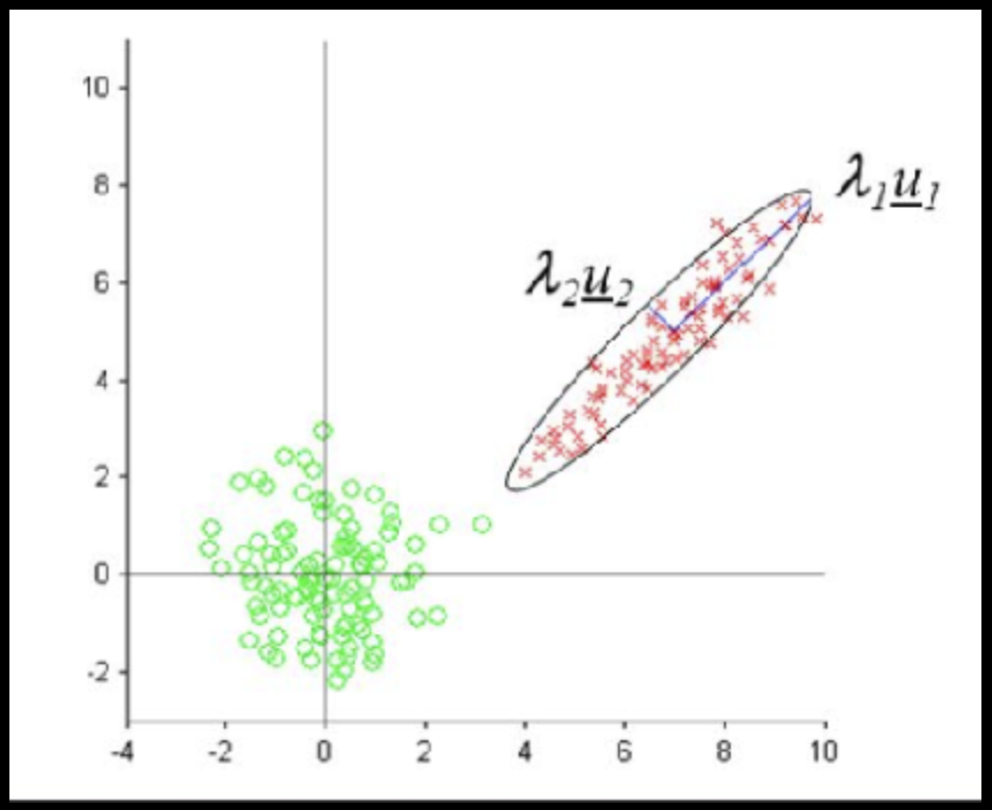
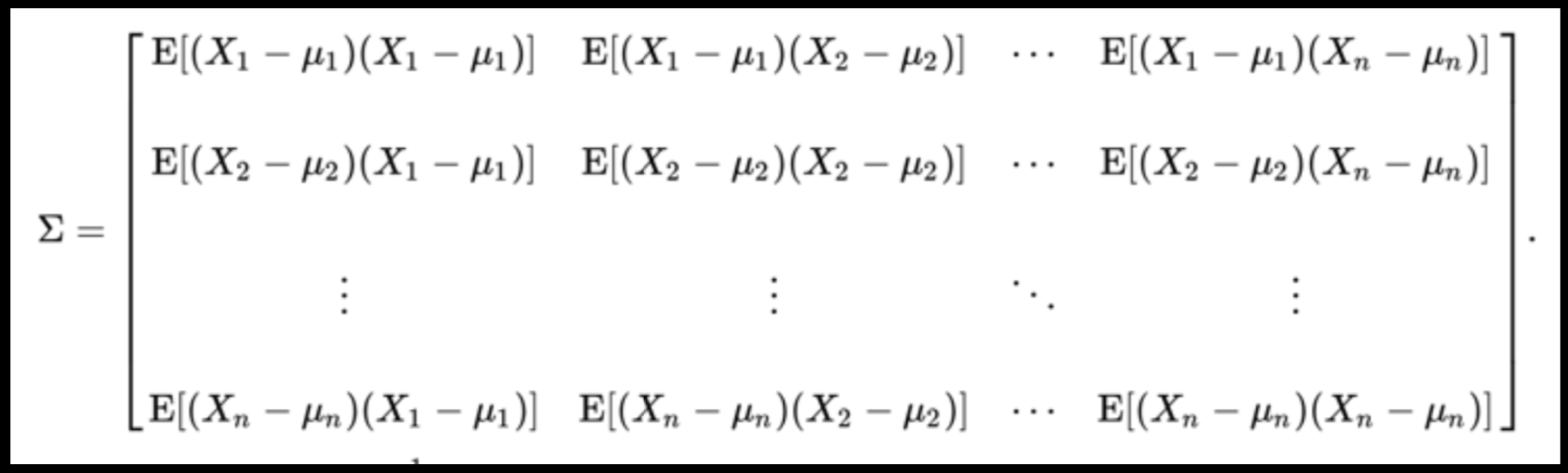
Data can have covariance (and it almost always does!)
PLUTO Manhattan data (42,000 x 15)
axis 1 -> features
axis 0 -> observations
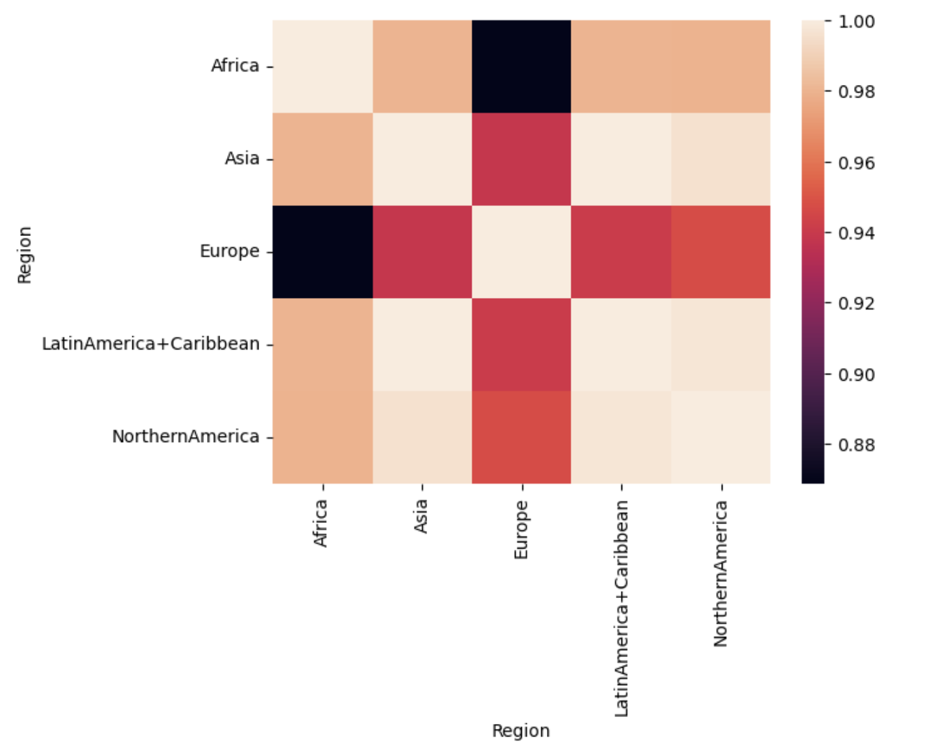
COVARIANCE = correlation / variance
Data can have covariance (and it almost always does!)
Data can have covariance (and it almost always does!)
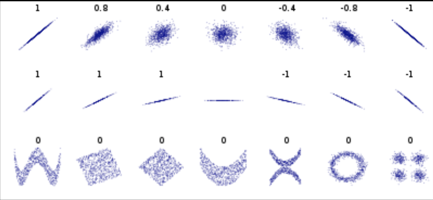
Pearson's correlation (linear correlation)
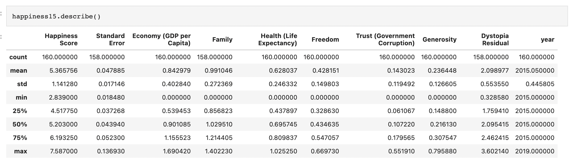
Generic preprocessing... WHY??
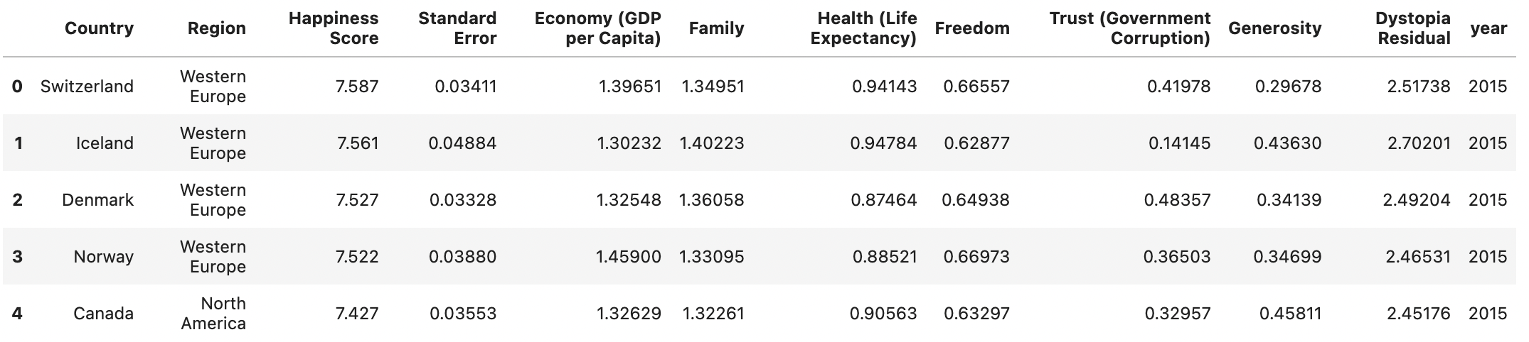
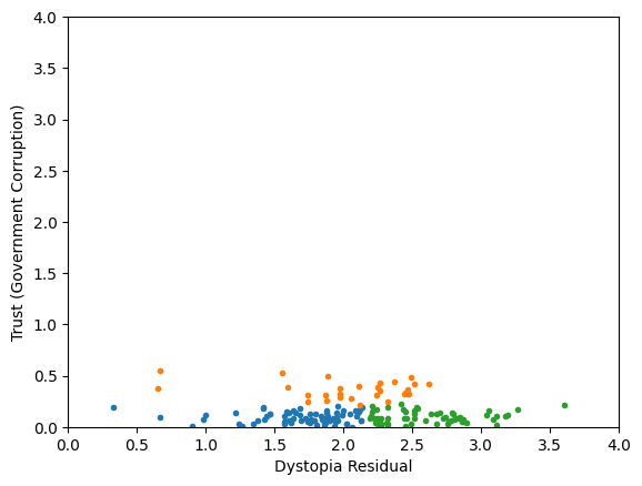
Worldbank Happyness Dataset https://github.com/fedhere/MLPNS_FBianco/blob/main/clustering/happiness_solution.ipynb
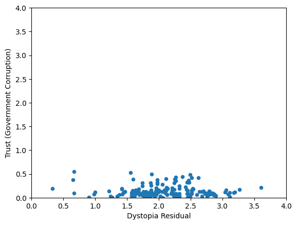
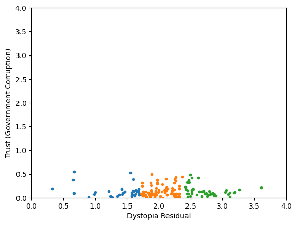
Clustering without scaling:
only the variable with more spread matters
Skewed data distribution:
std(x) ~ range(y)
Generic preprocessing... WHY??
Worldbank Happyness Dataset https://github.com/fedhere/MLPNS_FBianco/blob/main/clustering/happiness_solution.ipynb
Clustering without scaling:
only the variable with more spread matters
Skewed data distribution:
std(x) ~ range(y)
Clustering
Classifying &
regression
Unsupervised learning
Supervised learning
unsupervised vs supervised learning
Data that is not correlated appear as a sphere in the Ndimensional feature space
Data can have covariance (and it almost always does!)
ORIGINAL DATA
STANDARDIZED DATA
Generic preprocessing
Generic preprocessing... WHY??
Worldbank Happyness Dataset
Classification/Clustering without scaling:
only the variable with more spread matters
Generic preprocessing... WHY??
Worldbank Happyness Dataset
Classification/Clustering without scaling:
only the variable with more spread matters
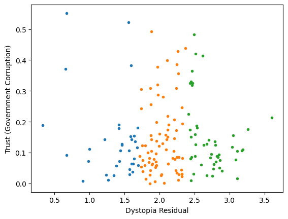
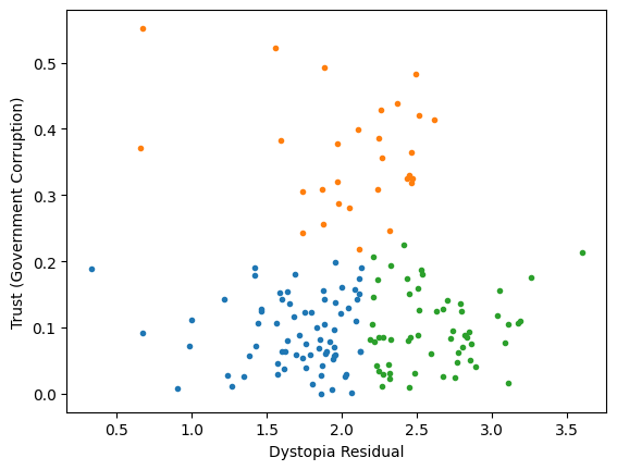
Classification/Clustering
after scaling:
both variables matter equally
Data that is not correlated appear as a sphere in the Ndimensional feature space
Data can have covariance (and it almost always does!)
ORIGINAL DATA
STANDARDIZED DATA
Generic preprocessing
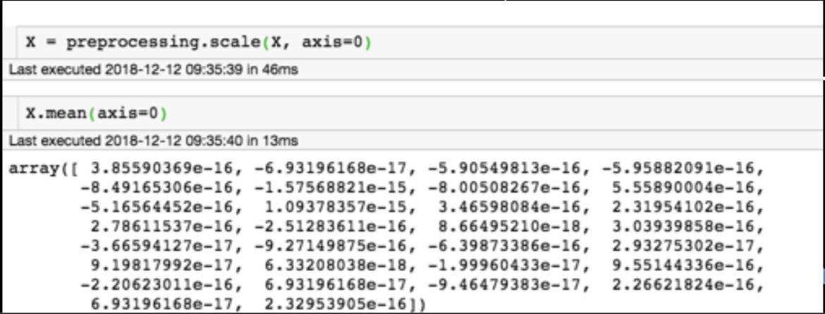
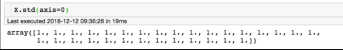
Generic preprocessing
for each feature: divide by standard deviation and subtract mean
Generic preprocessing: most commonly, we will just correct for the spread and centroid
The term "whitening" refers to white noise, i.e. noise with the same power at all frequencies"
PLUTO Manhattan data (42,000 x 15) correlation matrix
axis 1 -> features
axis 0 -> observations
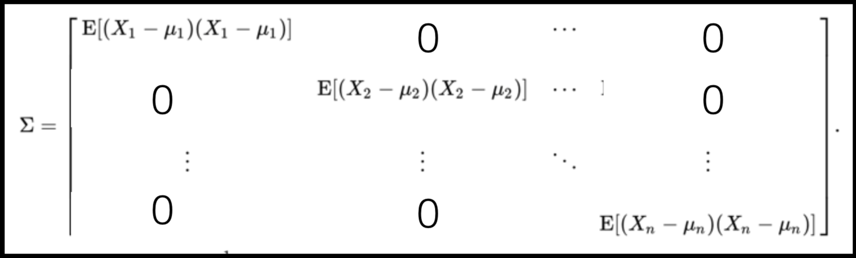
Data can have covariance (and it almost always does!)
PLUTO Manhattan data (42,000 x 15) correlation matrix
A covariance matrix is diagonal if the data has no correlation
Data can have covariance (and it almost always does!)
Full On Whitening
find the matrix W that diagonalized Σ
from zca import ZCA
import numpy as np
X = np.random.random((10000, 15)) # data array
trf = ZCA().fit(X)
X_whitened = trf.transform(X)
X_reconstructed =
trf.inverse_transform(X_whitened)
assert(np.allclose(X, X_reconstructed))
: remove covariance by diagonalizing the transforming the data with a matrix that diagonalizes the covariance matrix
this is at best hard, in some cases impossible even numerically on large datasets
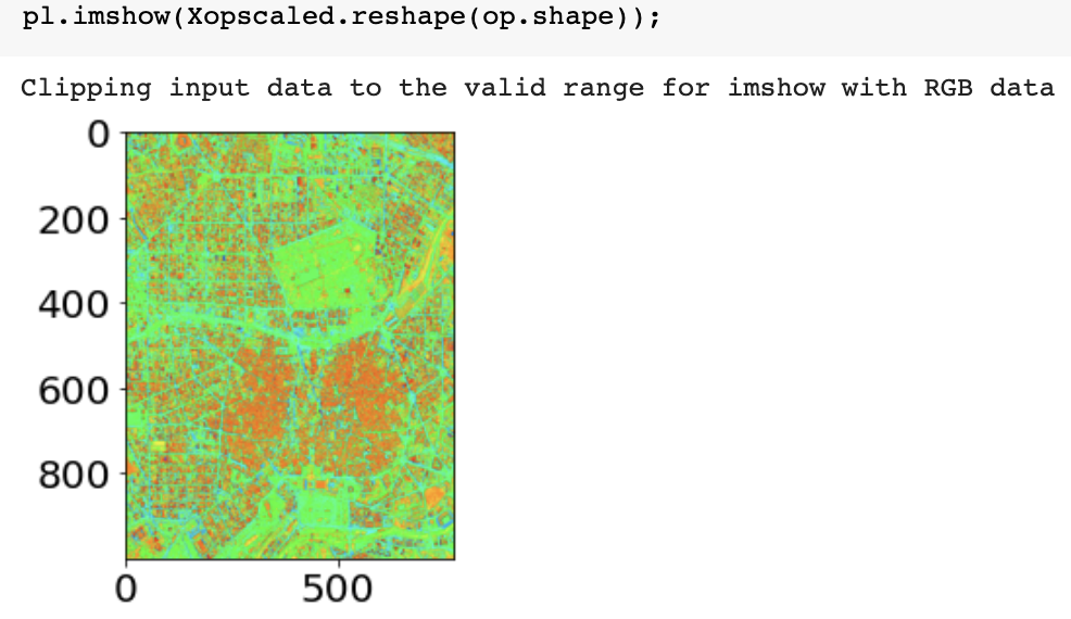
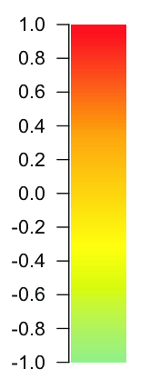
Generic preprocessing: other common schemes
for image processing (e.g. segmentation) often you need to mimmax preprocess
from sklearn import preprocessing

Xopscaled = preprocessing.minmax_scale(image_pixels.astype(float), axis=1)
Xopscaled.reshape(op.shape)[200, 700]
before
after (looks the same but colorbar different)
-107
273
0
1
the algorithm: Stochastic Gradient Descent (SGD)
assume a simpler line model y = ax
(b = 0) so we only need to find the "best" parameter a
the algorithm: Stochastic Gradient Descent
assume a simpler line model y = ax
(b = 0) so we only need to find the "best" parameter a
1. choose initial value for a
-1
the algorithm: Stochastic Gradient Descent
assume a simpler line model y = ax
(b = 0) so we only need to find the "best" parameter a
1. choose initial value for a
2. calculate the SSE
the algorithm: Stochastic Gradient Descent
assume a simpler line model y = ax
(b = 0) so we only need to find the "best" parameter a
1. choose initial value for a
2. calculate the SSE
3. calculate best direction to go to decrease the SSE
the algorithm: Stochastic Gradient Descent
assume a simpler line model y = ax
(b = 0) so we only need to find the "best" parameter a
1. choose initial value for a
2. calculate the SSE
3. calculate best direction to go to decrease the SSE
the algorithm: Stochastic Gradient Descent
assume a simpler line model y = ax
(b = 0) so we only need to find the "best" parameter a
1. choose initial value for a
2. calculate the SSE
3. calculate best direction to go to decrease the SSE
the algorithm: Stochastic Gradient Descent
assume a simpler line model y = ax
(b = 0) so we only need to find the "best" parameter a
1. choose initial value for a
2. calculate the SSE
3. calculate best direction to go to decrease the SSE
4. step in that direction
the algorithm: Stochastic Gradient Descent
assume a simpler line model y = ax
(b = 0) so we only need to find the "best" parameter a
1. choose initial value for a
2. calculate the SSE
3. calculate best direction to go to decrease the SSE
4. step in that direction
5. go back to step 2 and repeat
the algorithm: Stochastic Gradient Descent
assume a simpler line model y = ax
(b = 0) so we only need to find the "best" parameter a
1. choose initial value for a
2. calculate the SSE
3. calculate best direction to go to decrease the SSE
4. step in that direction
5. go back to step 2 and repeat
the algorithm: Stochastic Gradient Descent
assume a simpler line model y = ax
(b = 0) so we only need to find the "best" parameter a
1. choose initial value for a
2. calculate the SSE
3. calculate best direction to go to decrease the SSE
4. step in that direction
5. go back to step 2 and repeat
the algorithm: Stochastic Gradient Descent
assume a simpler line model y = ax
(b = 0) so we only need to find the "best" parameter a
1. choose initial value for a
2. calculate the SSE
3. calculate best direction to go to decrease the SSE
4. step in that direction
5. go back to step 2 and repeat
the algorithm: Stochastic Gradient Descent
assume a simpler line model y = ax
(b = 0) so we only need to find the "best" parameter a
1. choose initial value for a
2. calculate the SSE
3. calculate best direction to go to decrease the SSE
4. step in that direction
5. go back to step 2 and repeat
the algorithm: Stochastic Gradient Descent
assume a simpler line model y = ax
(b = 0) so we only need to find the "best" parameter a
1. choose initial value for a
2. calculate the SSE
3. calculate best direction to go to decrease the SSE
4. step in that direction
5. go back to step 2 and repeat
the algorithm: Stochastic Gradient Descent
for a line model y = ax + b
we need to find the "best" parameters a and b
1. choose initial value for a & b
2. calculate the SSE
3. calculate best direction to go to decrease the SSE
4. step in that direction
5. go back to step 2 and repeat
the algorithm: Stochastic Gradient Descent
for a line model y = ax + b
we need to find the "best" parameters a and b
1. choose initial value for a & b
2. calculate the SSE
3. calculate best direction to go to decrease the SSE
4. step in that direction
5. go back to step 2 and repeat
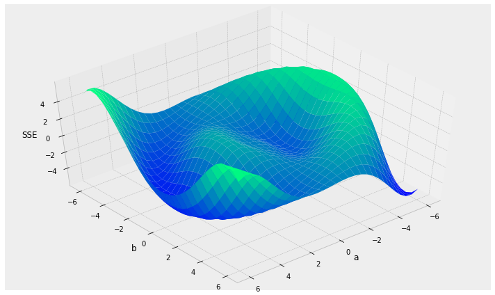
the algorithm: Stochastic Gradient Descent
Things to consider:
the algorithm: Stochastic Gradient Descent
Things to consider:
- local vs. global minima
local minima
global minimum
the algorithm: Stochastic Gradient Descent
Things to consider:
- local vs. global minima
- initialization: choosing starting spot?
global minimum
local minima
the algorithm: Stochastic Gradient Descent
Things to consider:
- local vs. global minima
- initialization: choosing starting spot?
- learning rate: how far to step?
the algorithm: Stochastic Gradient Descent
Things to consider:
- local vs. global minima
- initialization: choosing starting spot?
- learning rate: how far to step?
- stopping criterion: when to stop?
the algorithm: Stochastic Gradient Descent
Things to consider:
- local vs. global minima
- initialization: choosing starting spot?
- learning rate: how far to step?
- stopping criterion: when to stop?
Stochastic Gradient Descent (SGD): use a different (random) sub-sample of the data at each iteration
By federica bianco


