


federica bianco PRO
astro | data science | data for good
Federica Bianco
University of Delaware
Rubin Observatory
this slide deck:
1
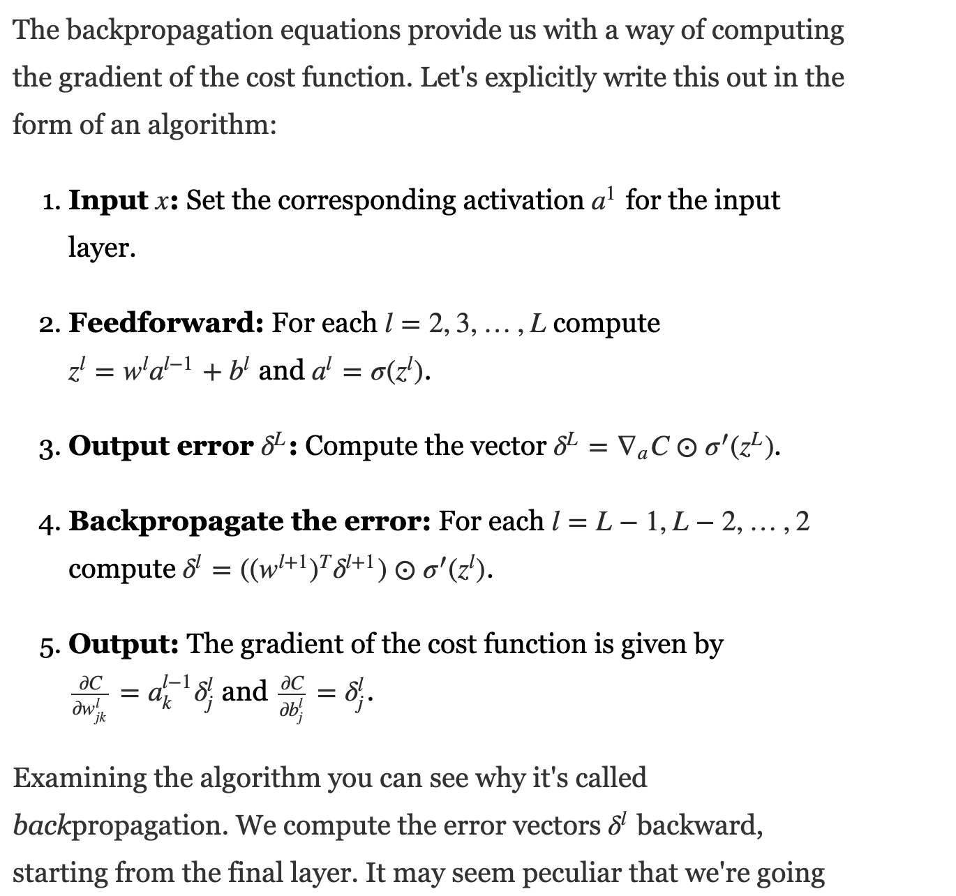
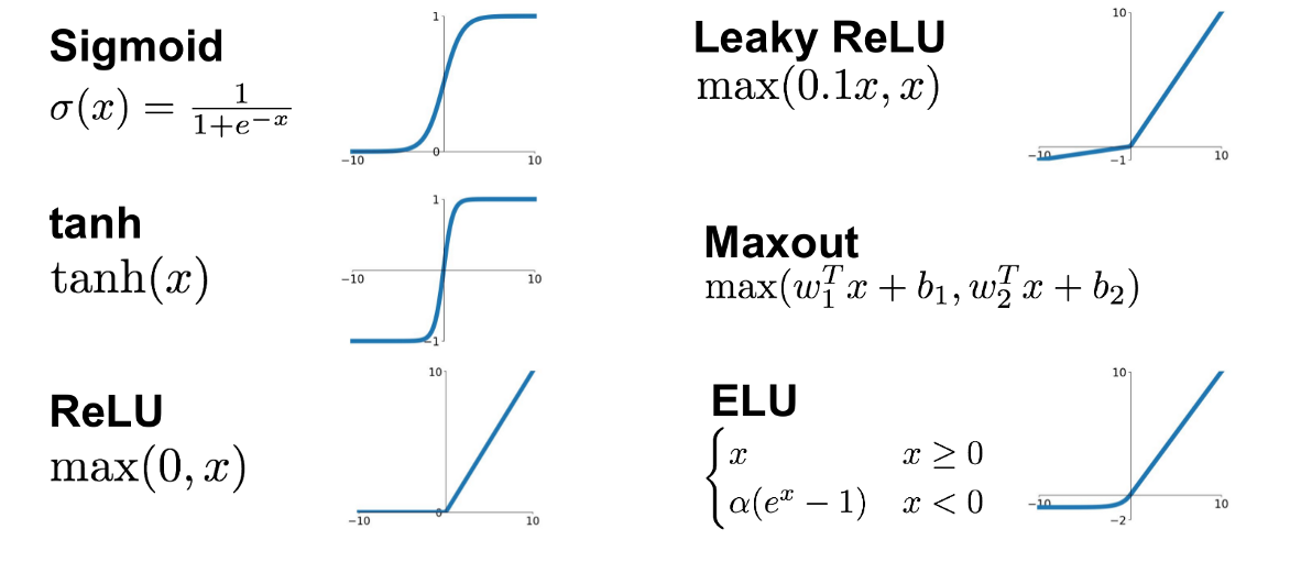
what we are doing, except for the activation function
is exactly a series of matrix multiplictions.
3x5
5x2
2x1
=
The purpose is to approximate a function φ
y = φ(x)
which (in general) is not linear with linear operations
what we are doing, except for the activation function
is exactly a series of matrix multiplictions.
.
.
.
Any linear model:
y : prediction
ytrue : target
Error: e.g.
intercept
slope
L2
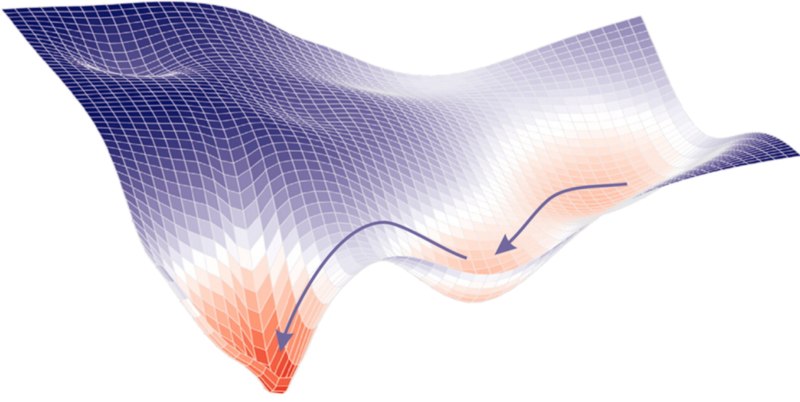
Find the best parameters by finding the minimum of the L2 hyperplane
at every step look around and choose the best direction
.
.
.
Any linear model:
y : prediction
ytrue : target
Error: e.g.
intercept
slope
L2
Find the best parameters by finding the minimum of the L2 hyperplane
at every step look around and choose the best direction
.
.
.
Any linear model:
y : prediction
ytrue : target
Error: e.g.
intercept
slope
L2
Find the best parameters by finding the minimum of the L2 hyperplane
at every step look around and choose the best direction
new position
.
.
.
Any linear model:
y : prediction
ytrue : target
Error: e.g.
intercept
slope
L2
Find the best parameters by finding the minimum of the L2 hyperplane
at every step look around and choose the best direction
old position
.
.
.
Any linear model:
y : prediction
ytrue : target
Error: e.g.
intercept
slope
L2
Find the best parameters by finding the minimum of the L2 hyperplane
at every step look around and choose the best direction
gradient at the old position
.
.
.
Any linear model:
y : prediction
ytrue : target
Error: e.g.
intercept
slope
L2
Find the best parameters by finding the minimum of the L2 hyperplane
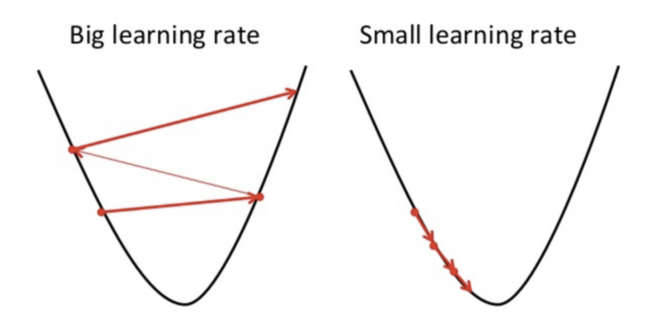
at every step look around and choose the best direction
learning rate
.
.
.
Any linear model:
Error: e.g.
learning rate
adaptive lr
how does linear descent look when you have a whole network structure with hundreds of weights and biases to optimize??
.
.
.
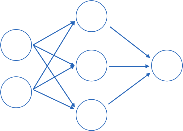
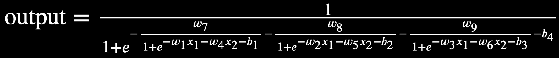
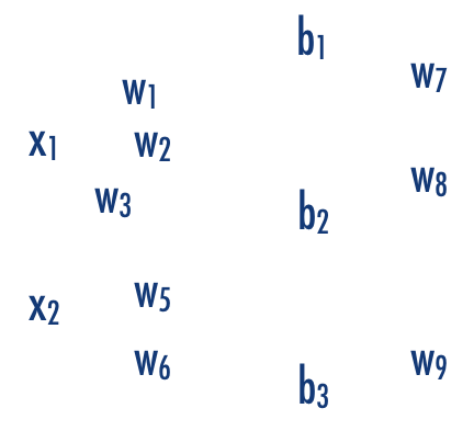
output
Training models with this many parameters requires a lot of care:
. defining the metric
. optimization schemes
. training/validation/testing sets
But just like our simple linear regression case, small changes in the parameters lead to small changes in the output for the right activation functions.
define a cost function, e.g.
x1
x2
b1
b2
b3
b
w11
w12
w13
w21
w22
w23
Training models with this many parameters requires a lot of care:
. defining the metric
. optimization schemes
. training/validation/testing sets
But just like our simple linear regression case, small changes in the parameters lead to small changes in the output for the right activation functions.
define a cost function, e.g.
Training models with this many parameters requires a lot of care:
. defining the metric
. optimization schemes
. training/validation/testing sets
But just like our simple linear regression case, the fact that small changes in the parameters leads to small changes in the output for the right activation functions.
define a cost function, e.g.
Training a DNN
feed data forward through network and calculate cost metric
for each layer, calculate effect of small changes on next layer
how does linear descent look when you have a whole network structure with hundreds of weights and biases to optimize??
think of applying just gradient to a function of a function of a function... use:
1) partial derivatives, 2) chain rule
define a cost function, e.g.
Training a DNN
at every step look around and choose the best direction
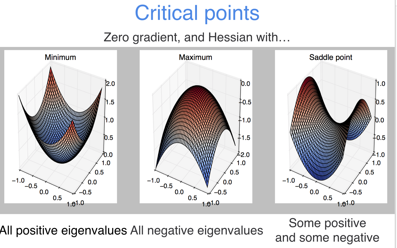
why do we not worry about local minima?
the course of dimensionality actually is a blessing here!
Time series analysis
2
Consider a dataset that is a time series
1D: exogenous-endogenous variable
temperature
y depend on x
brightness
Consider a dataset that is a time series
1D: exogenous-endogenous variable
time
y depend on x
brightness
Consider a dataset that is a time series
1D: exogenous-endogenous variable
time
y depend on x
exogenous variable is sequencial
time has an directionality:
y(t+1) depends on y(t)
brightness
A time series is any measurable quantity sampled at multiple points in time.
Time series are series of exogenous-endogenous variable pairs where the exogenous variable is time, and therefore it is a sequential quantity with a specific direction of evolution.
Key Concept
Evenly vs Unevenly sampled time series.
Most statistical methods are developed for evenly sampled TS.
Most physical TS are unevenly sampled
time
time
evenly: dt is constant
unevenly: dt changes
Unusally time of sampling is known
time
time
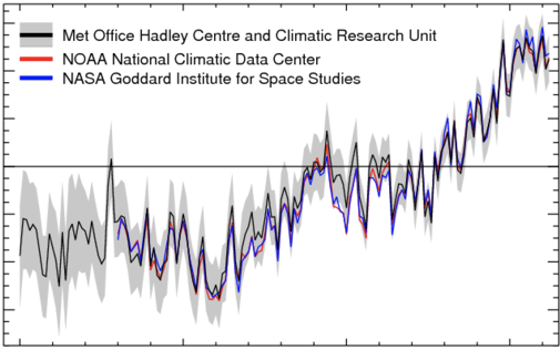
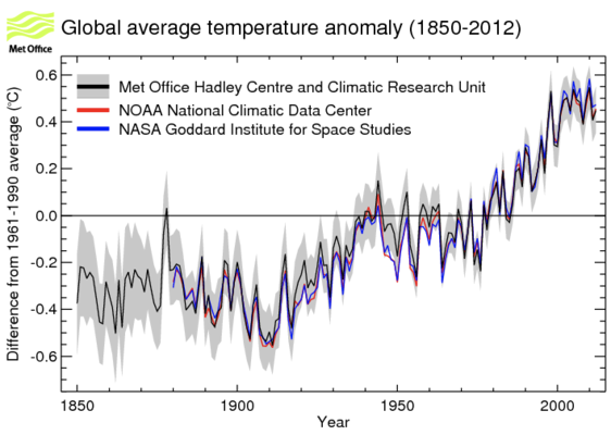
what is interesting in this time series?
what is interesting in this time series?
trend
what is interesting in this time series?
what is interesting in this time series?
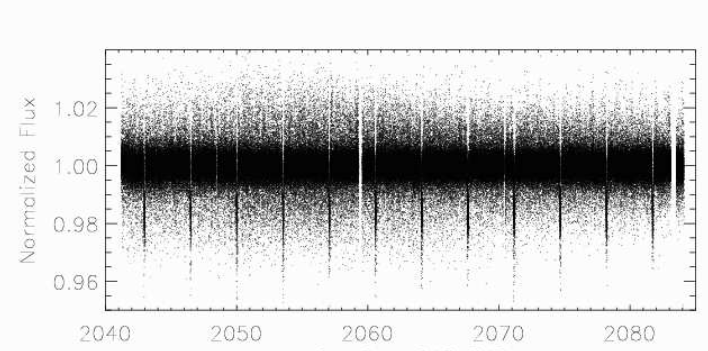
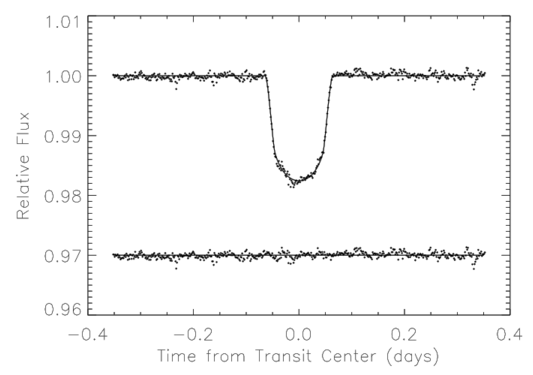
periodicity (repetitive patterns)
HD 209458, the first transiting planet to be discovered.
what is interesting in this time series?
periodicity (repetitive patterns)
HD 209458, the first transiting planet to be discovered.
"optimal" Folding is a common methodology to detect periods
what is interesting in this time series?
what is interesting in this time series?
events
what is interesting in this time series?
events
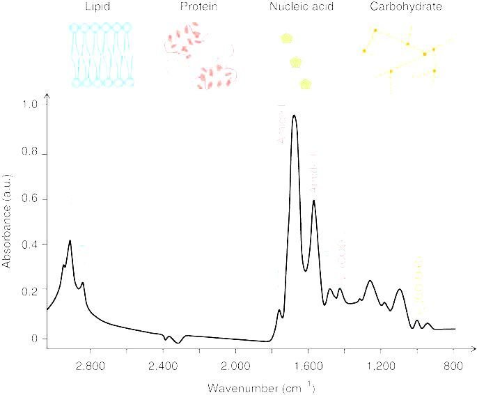
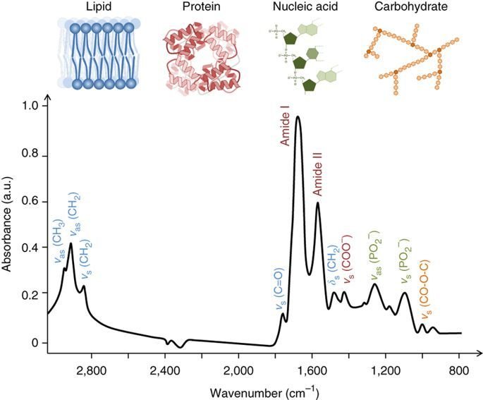
this is not a "time" series, but a spectral series, but it is still a 1-D dataset with directional exogenous variable so the same methodologies can be applied
what is interesting in this time series?
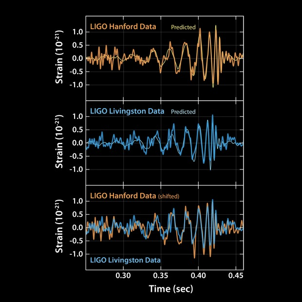
event detection/template matching
LIGO gravitational wave detection
Abbott et al. Physical Review Letters 116, 061102 (2016)
what is interesting here?
event detection
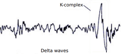
what is interesting here?
event detection
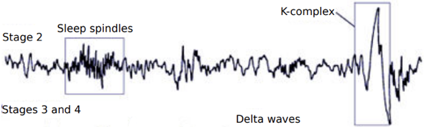
The 3 behavioral states of wakefulness, rapid eye movement (REM) sleep, and non-REM (NREM)
sleep are characterized by specific changes in electroencephalography,
what is interesting here?
Point of change detection
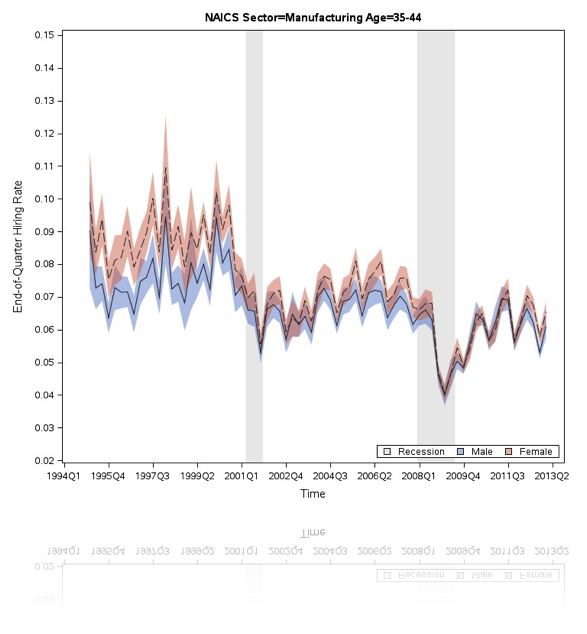
Longitudinal Employer-Household Dynamics
what is interesting here?
Longitudinal Employer-Household Dynamics
seasonal variations,
cyclic variation,
periodicity
what is interesting here?
TSA topics
unobserved state
Underlying state x is a time varying Markovian process (the position of the pace craft)
The observed variable depends at least on the state and on noise.
Other elements (e.g. seasonality) can be included in the model too
we can write a Bayesian structural model like this:
local level
state
seasonal trend
we can write a Bayesian structural model like this:
seasonal variations
unobserved trend
Its a Markovian Process:
stochastic process with 1-step memory
there is a hidden or latent process xt called the state process (the position of the space craft)
Training a DNN
1994
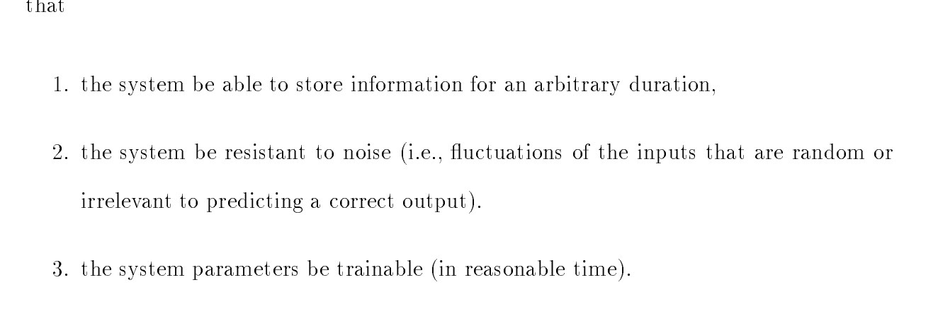
An time-domain enabled AI system should:
Training a DNN
you need to pick
t
1994
Training a DNN
you need to pick
Training a DNN
1994
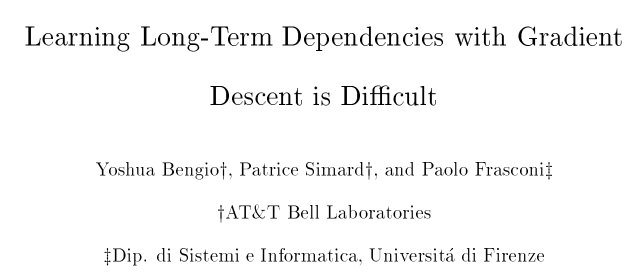
We show why gradient based learning algorithms face an increasingly dicult problem as the duration of the dependencies to be captured increases
the magnitude of the derivative of the state of a dynamical system at time t with respect to the state at time 0 decreases exponentially as t increases.
We show why gradient based learning algorithms face an increasingly dicult problem as the duration of the dependencies to be captured increases
you need to pick
Training a DNN
you need to pick
Training a DNN
1994
RNN
3
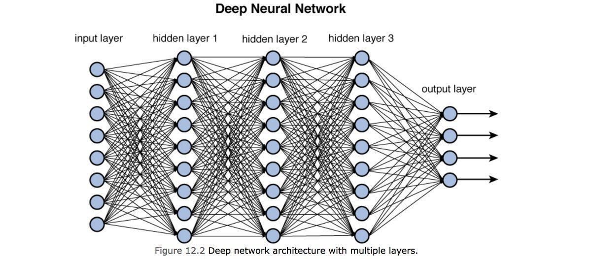
RNN architecture
input layer
output layer
hidden layers
Feed-forward NN architecture
RNN architecture
output layer
hidden layers
Recurrent NN architecture
input layer
output layer
RNN hidden layers
output layer
hidden layers
input layer
Feed-forward NN architecture
RNN architecture
input layer
output layer
RNN hidden layers
current state
previous state
In TSA this is a State Space Probem
we want process a sequence of vectors x applying a recurrence formula at every time step:
current input
RNN architecture
input layer
output layer
RNN hidden layers
current state
features
(can be time dependent)
function with parameters q
In TSA this is a State Space Probem
we want process a sequence of vectors x applying a recurrence formula at every time step:
previous state
A State-space model is a model to derive the value of a time-dependent variable x(t), the state, generated by a noisy Markovian process, from observations of a variable y(t), also subject to noise, linearly related to the target variable
Definition
RNN architecture
input layer
output layer
RNN hidden layers
Simplest possible RNN
Whh
Wxh
Qhy
RNN architecture
input layer
output layer
RNN hidden layers
Simplest possible RNN
Whh
Wxh
Qhy
RNN architecture
input layer
Alternative graphical representation of RNN
h(t-1)
h(t)
h(t+1)
h(t+2)
h(t+3)
h(t+4)
y(t)
y(t+1)
y(t+2)
y(t+4)
y(t+3)
y(t+5)
Qhy
Whh
Whh
Whh
Whh
Whh
Wxh
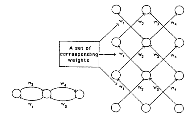
the weights are the same! always the same Whh and Qhy
Qhy
Qhy
Qhy
Qhy
RNN architecture
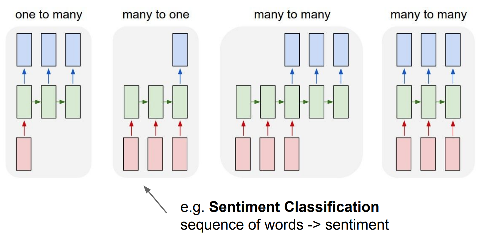
applications
image captioning:
one image to a
sequence of words
RNN architecture
appllications
image captioning:
one image to a
sequence of words
sentiment analysis
sequence of words to one sentiment
RNN architecture
appllications
image captioning:
one image to a
sequence of words
sentiment analysis
sequence of words to one sentiment
language translator
sequence of words to sequence of words
RNN architecture
appllications
image captioning:
one image to a
sequence of words
sentiment analysis
sequence of words to one sentiment
language translator
sequence of words to sequence of words
online: video classification frame by frame
RNN architecture
more complicated RNNs
Some layers will be recurrent, others will not. Does not need to be fully connected
RNN architecture
input layer
e(t)
h(t-1)
h(t)
h(t+1)
h(t+2)
h(t+3)
h(t+4)
y(t)
y(t+1)
y(t+2)
y(t+4)
y(t+3)
y(t+5)
Why
Why
Why
Why
Why
Whh
Whh
Whh
Whh
Whh
Wxh
each output has its own loss
Why
e(t+1)
e(t+2)
e(t+3)
e(t+4)
e(t+5)
RNN architecture
input layer
e(t)
h(t-1)
h(t)
h(t+1)
h(t+2)
h(t+3)
h(t+4)
y(t)
y(t+1)
y(t+2)
y(t+4)
y(t+3)
y(t+5)
Why
Why
Why
Why
Why
Whh
Whh
Whh
Whh
Whh
Wxh
each output has its own loss
Why
e(t+1)
e(t+2)
e(t+3)
e(t+4)
e(t+5)
The cats that ate were full
The cat that ate was full
RNN architecture
input layer
e(t)
h(t-1)
h(t)
h(t+1)
h(t+2)
h(t+3)
h(t+4)
y(t)
y(t+1)
y(t+2)
y(t+4)
y(t+3)
y(t+5)
Why
Why
Why
Why
Why
Whh
Whh
Whh
Whh
Whh
Wxh
each output has its own loss
Why
e(t+1)
e(t+2)
e(t+3)
e(t+4)
e(t+5)
LOSS
RNN architecture
input layer
e(t)
h(t-1)
h(t)
h(t+1)
h(t+2)
h(t+3)
h(t+4)
y(t)
y(t+1)
y(t+2)
y(t+4)
y(t+3)
y(t+5)
Why
Why
Why
Why
Why
Whh
Whh
Whh
Whh
Whh
Wxh
each output has its own loss
Why
e(t+1)
e(t+2)
e(t+3)
e(t+4)
e(t+5)
Total loss:
RNN architecture
input layer
h(t-1)
h(t)
h(t+1)
h(t+2)
h(t+3)
h(t+4)
y(t)
y(t+1)
y(t+2)
y(t+4)
y(t+3)
Why
Why
Why
Why
Why
Whh
Whh
Whh
Whh
Whh
Wxh
each output has its own loss
Why
Total loss:
e(t)
y(t+5)
e(t+1)
e(t+2)
e(t+3)
e(t+4)
e(t+5)
RNN architecture
input layer
h(t-1)
h(t)
h(t+1)
h(t+2)
h(t+3)
h(t+4)
y(t)
y(t+1)
y(t+2)
y(t+4)
y(t+3)
Why
Why
Why
Why
Why
Whh
Whh
Whh
Whh
Whh
Wxh
each output has its own loss
Why
Total loss:
e(t)
y(t+5)
e(t+1)
e(t+2)
e(t+3)
e(t+4)
e(t+5)
RNN architecture
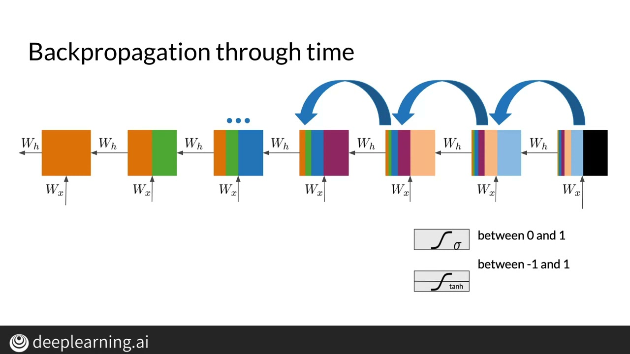
vanishing gradient problem!
input layer
h(t-1)
h(t)
h(t+1)
h(t+2)
h(t+3)
h(t+4)
y(t)
y(t+1)
y(t+2)
y(t+4)
y(t+3)
y(t+5)
Why
Why
Why
Why
Why
Whh
Whh
Whh
Whh
Whh
Wxh
Why
obsesses
over
recent
past
forgets
remote
past
vanishing gradient problem!
input layer
e(t)
h(t-1)
h(t)
h(t+1)
h(t+2)
h(t+3)
h(t+4)
y(t)
y(t+1)
y(t+2)
y(t+4)
y(t+3)
y(t+5)
Why
Why
Why
Why
Why
Whh
Whh
Whh
Whh
Whh
Wxh
Why
e(t+1)
e(t+2)
e(t+3)
e(t+4)
e(t+5)
vanishing gradient problem is exacerbated by having the same set of weights.
The vanishing gradient problem causes early layer to not to learn as effectively
The earlier layers learn from the remote past
As a result: vanilla RNN would only have short term memory (only learn from recent states)
Whh
Whh
Whh
Whh
Whh
LSTM
4
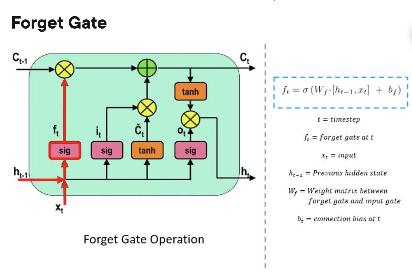
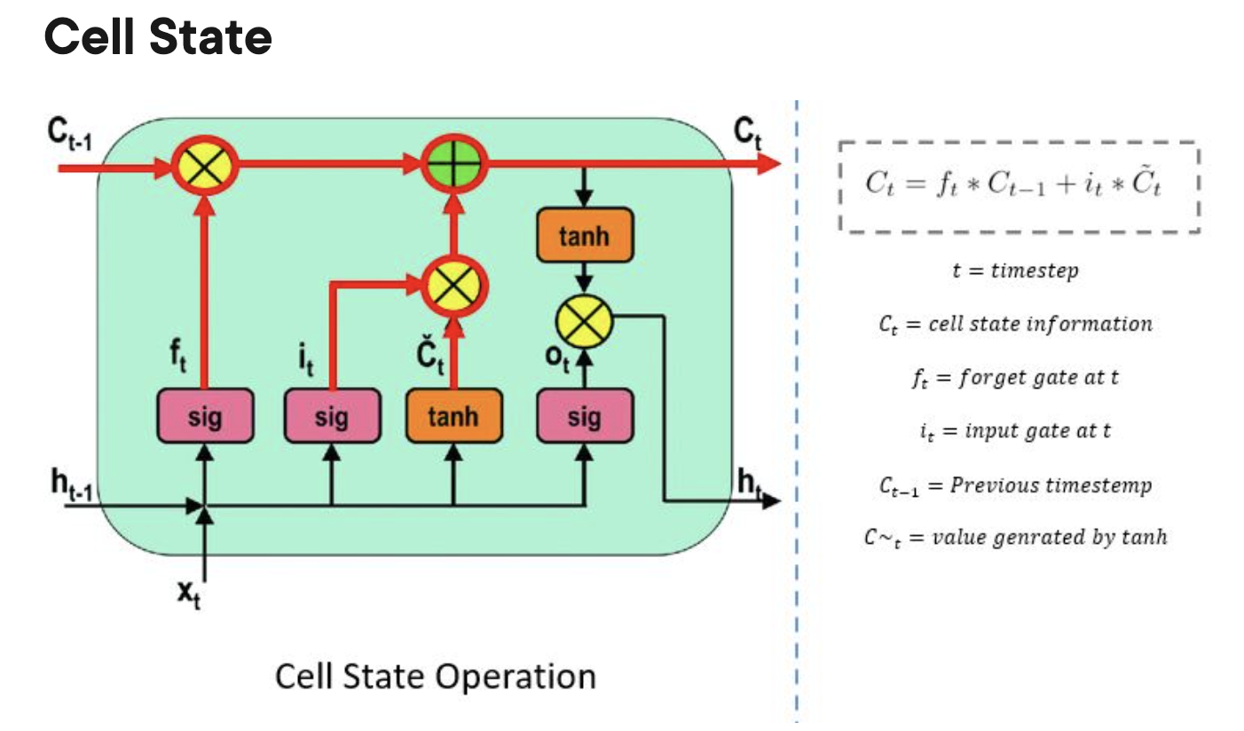
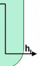
Ct: output
h: hidden states
X: input
Ct-1 : previous cell state (previous output)
ht-1 : previous hidden state
xt : current state (input)
forget gate:
do i keep memory of this past step
LSTM: long short term memory
solution to the vanishing gradient problem
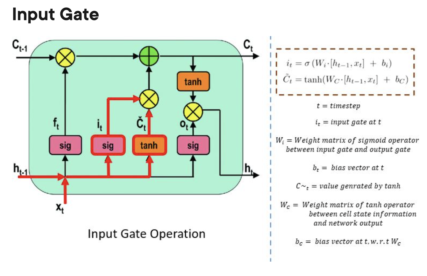
input gate:
do I update the current cell?
LSTM: long short term memory
solution to the vanishing gradient problem
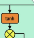
cell state:
procuces the prediction
LSTM: long short term memory
solution to the vanishing gradient problem
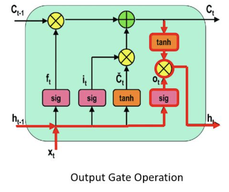
output gate
previous input that goes into the hidden state
LSTM: long short term memory
solution to the vanishing gradient problem
hidden state
produces the new hidden states
LSTM: long short term memory
solution to the vanishing gradient problem
LSTM: long short term memory
solution to the vanishing gradient problem
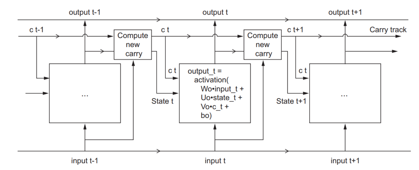
even if you want to predict a single time series, you need many example
split the time series into chunks
LSTM: how to actually run it
batch size: how many sequencies you pass at once
timeseries: how many time stamps in a sequence
features: how many measurements in the time seris
even if you want to predict a single time series, you need many example
split the time series into chunks
LSTM: how to actually run it
batch size: N
timeseries: 50000
features: 2
model = Sequential()
model.add(LSTM(32, input_shape=(1000, 2)))
model.add(Dense(2))
even if you want to predict a single time series, you need many example
split the time series into chunks
LSTM: how to actually run it
To be or not to be? this is the question. Whether 'tis nobler in the mind
sequencies of 12 letters
batch size: N
timeseries: 12
features: 1
LSTM: how to actually run it
A fun notebook: create new paper titles (takes a lot to train tho so we cannot do it in class)
visualizing NNs
5
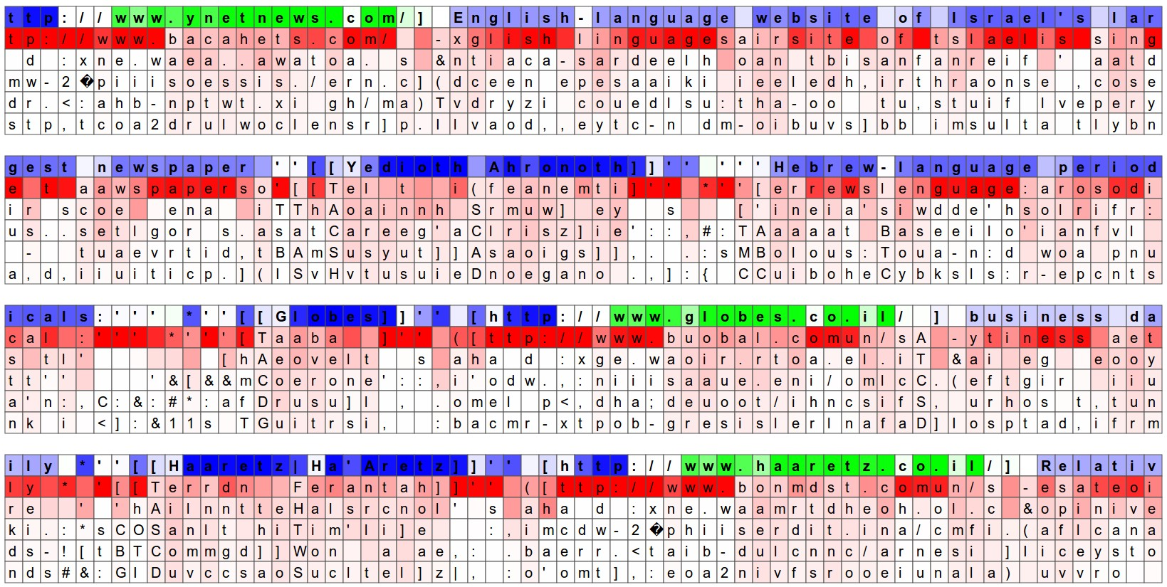
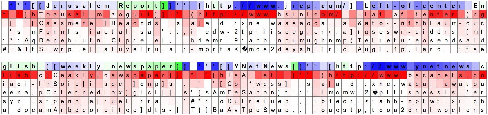
Saliency Maps
"The guesses are colored by their probability (so dark red = judged as very likely, white = not very likely).
...
The input character sequence (blue/green) is colored based on the firing of a randomly chosen neuron in the hidden representation of the RNN. Think about it as green = very excited and blue = not very excited (... these are values between [-1,1] in the hidden state vector, which is just the gated and tanh’d LSTM cell state).
Intuitively, this is visualizing the firing rate of some neuron in the “brain” of the RNN while it reads the input sequence. Different neurons might be looking for different patterns.
learning markdown syntax: URL's
learning markdown syntax: [[]]
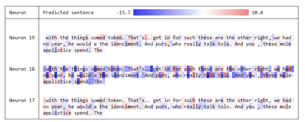
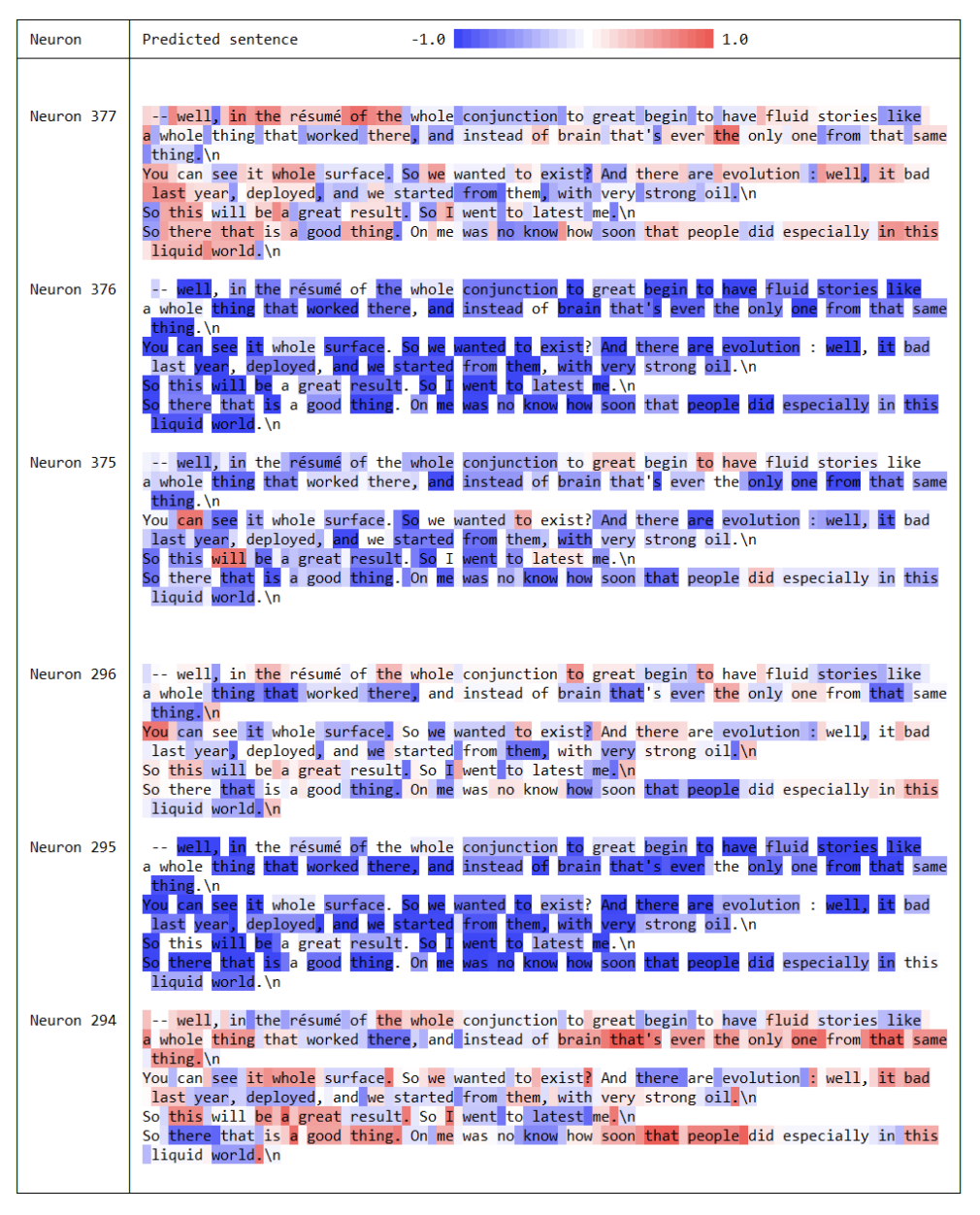
"The guesses are colored by their probability (so dark red = judged as very likely, white = not very likely).
...
The input character sequence (blue/green) is colored based on the firing of a randomly chosen neuron in the hidden representation of the RNN. Think about it as green = very excited and blue = not very excited (... these are values between [-1,1] in the hidden state vector, which is just the gated and tanh’d LSTM cell state).
Intuitively, this is visualizing the firing rate of some neuron in the “brain” of the RNN while it reads the input sequence. Different neurons might be looking for different patterns.
Vanilla RNN
LSTM
andrej karpathy
http://karpathy.github.io/2015/05/21/rnn-effectiveness/
Neural Network and Deep Learning
an excellent and free book on NN and DL
http://neuralnetworksanddeeplearning.com/index.html
Deep Learning An MIT Press book in preparation
Ian Goodfellow, Yoshua Bengio and Aaron Courville
https://www.deeplearningbook.org/lecture_slides.html
History of NN
https://cs.stanford.edu/people/eroberts/courses/soco/projects/neural-networks/History/history2.html
By federica bianco
Autoencoders and RNNs


