


federica bianco PRO
astro | data science | data for good
State Space Models and Bayesian Analysis
Fall 2025 - UDel PHYS 641
dr. federica bianco
@fedhere
combinatorial statistics
Bayes' theorem
optimization
gradient descent
stochastic gradient descent
Ockham's razor
Information theoory
AIC BIC MDL
MCMC
space state models for time series analysis
BSTS fitting
this slide deck:
machine learning standard practices
1
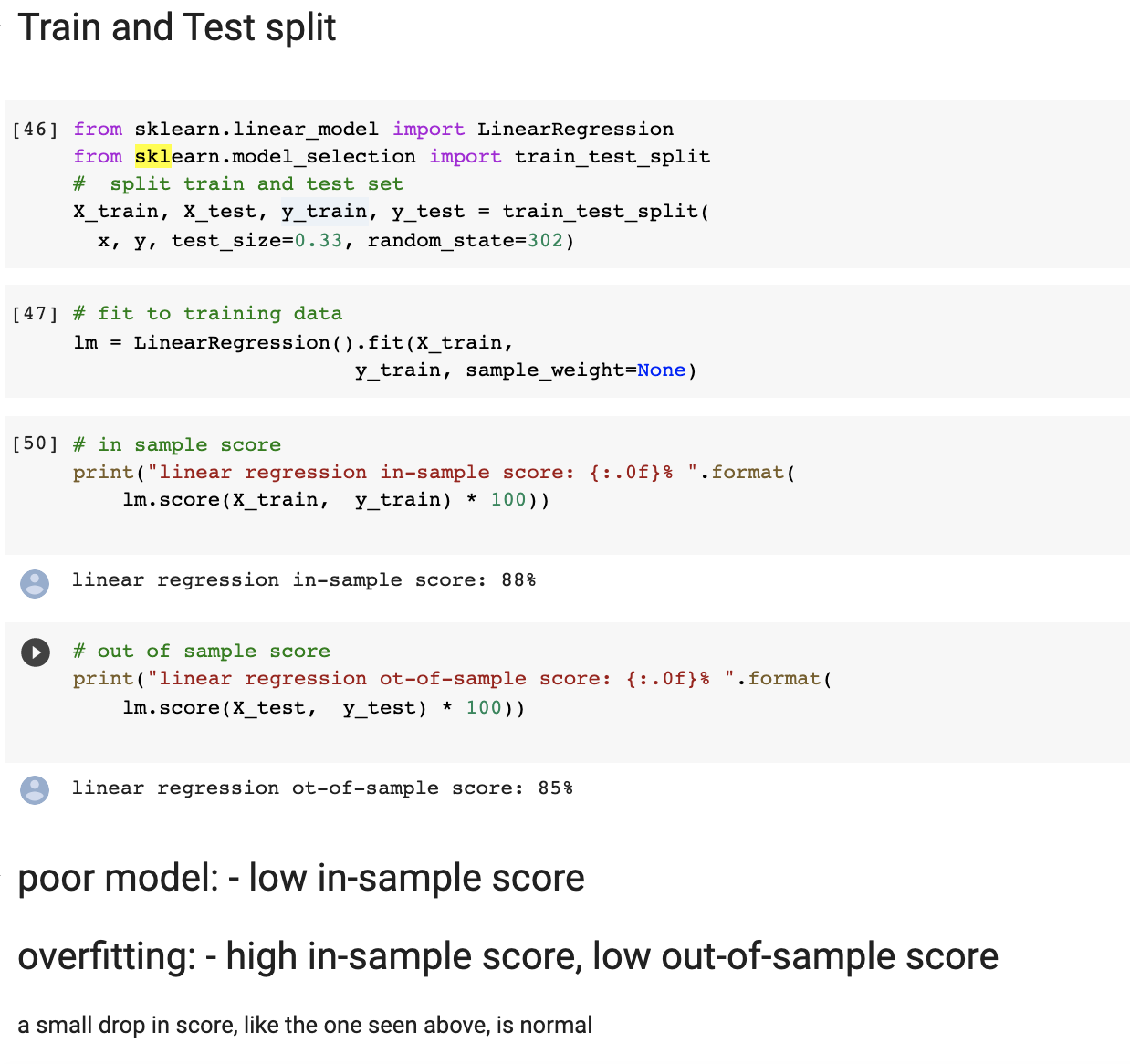
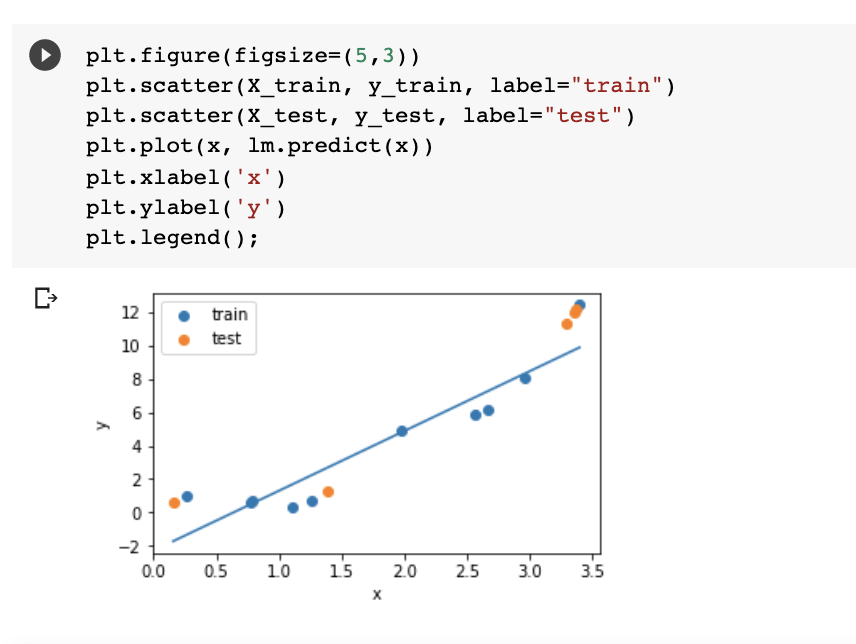
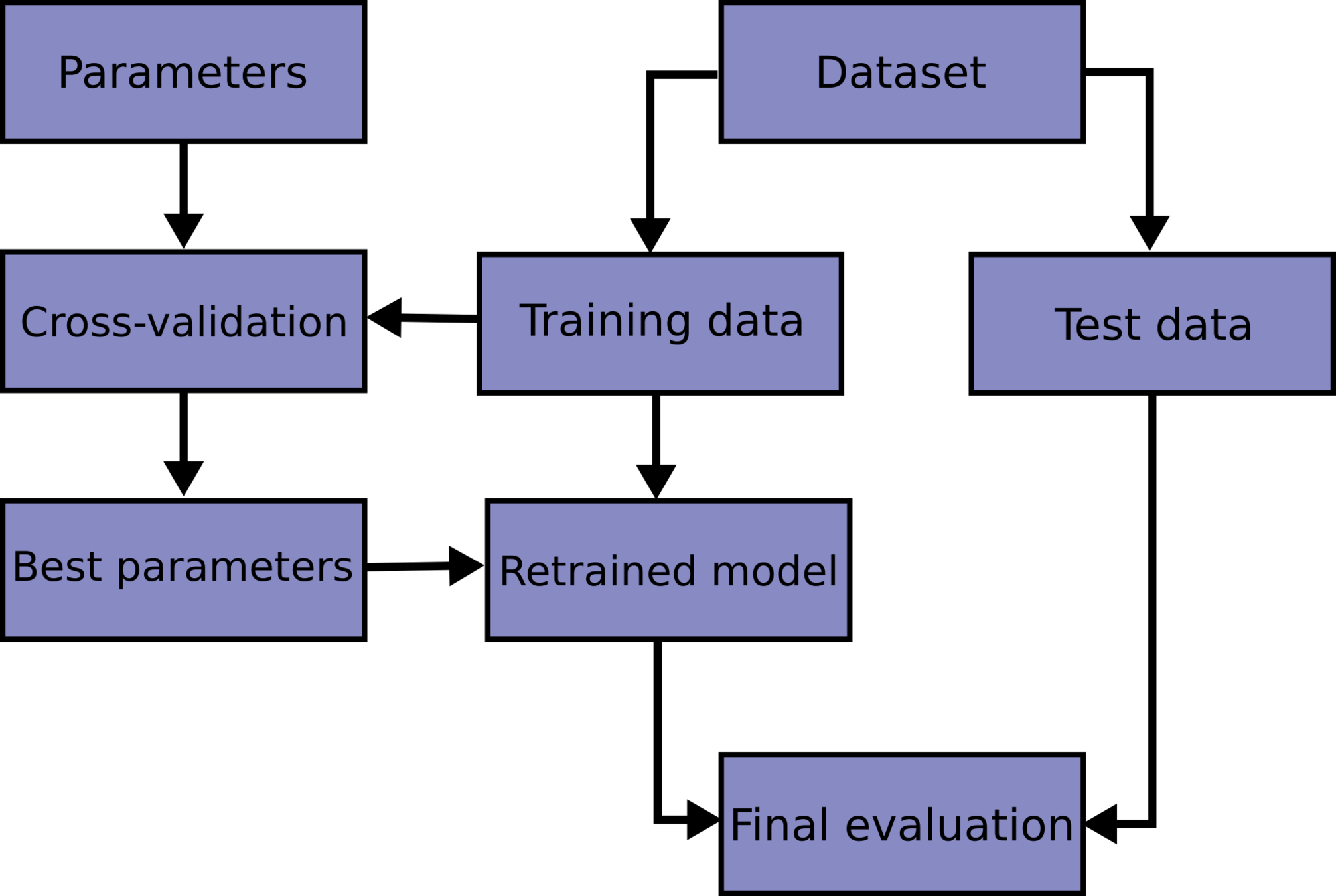
test train validation
train parameters on training set
run only once on the test set to assess the model performance
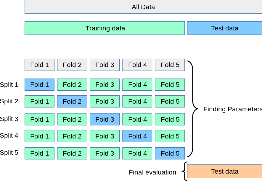
test + train + validation
train parameters on training set
adjust parameters on validation set
run only once on the test set to assess the model performance
k-fold cross validation
math and vis for your review
1.1
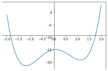
Target Funcion
Univariate Linear regression
b
a
Target Funcion
Univariate Linear regression
b
a
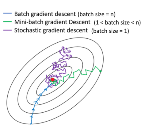
Add stochasticity to avoid getting stuck in a local minimum
stochastic gradient descent algorithm
"convergence" is reached when the gradient is ~0: with ε tollrance
stochastic gradient descent algorithm
"convergence" is reached when the gradient is ~0: with ε tollrance
Target Funcion
Univariate Linear regression
Stochastic Gradient Descent
where i 1 elements of the full N-dimensional observation set (a subset)
Target Funcion
Univariate Linear regression
b
a
idea 2. start a bunch of parallel optimizations
(we will see it in next class)
Correlation
1.2
formal definition of correlation function
probability and statistics
Crush Course in Statistics
freee statistics book: http://onlinestatbook.com/
descriptive statistics:
we summarize the proprties of a distribution
descriptive statistics
<=>
fraction of times something happens
probability of it happening
P(obs|model) = P(model|obs)
<=>
A DISTRIBUTION
The ratio of occurrency of values:
if I had infinite coin tasses what fraction of times would I get heads vs tails
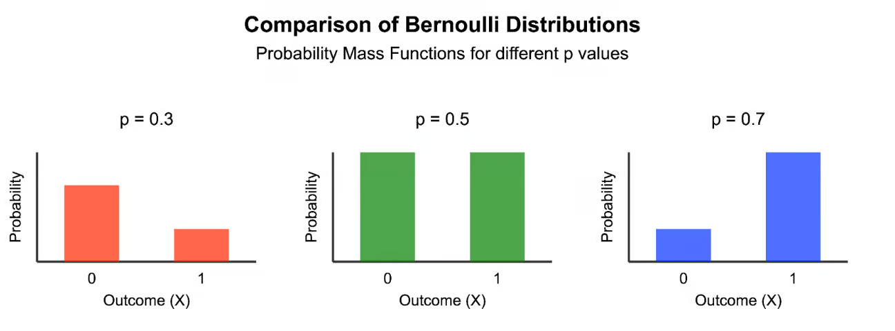
Coin toss => Bernoulli distribution
p(tail) = 0.5
fraction of times something happens
probability of it happening
P(obs|model) = P(model|obs)
represents a level of certainty relating to a potential outcome or idea:
if I believe the coin is unfair (tricked) then even if I get a head and a tail I will still believe I am more likely to get heads than tails
<=>
fraction of times something happens
probability of it happening
P(obs|model) = P(model|obs)
fraction of times something happens
probability of it happening
<=>
P(obs|model)/ P(model) = P(model|obs) / P(obs)
Coin toss => Bernoulli distribution
p(tail) = 0.3
p(tail) = 0.5
P(obs|model) = P(model|obs)
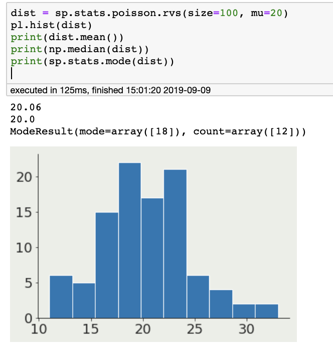
Descriptive Statistics deals with the characterization of distributions
descriptive statistics:
we summarize the proprties of a distribution
mean: n=1
other measures of centeral tendency:
median: 50% of the distribution is to the left,
50% to the right
mode: most popular value in the distribution
The moments of a distribution
central tendency (n=1)
descriptive statistics:
we summarize the proprties of a distribution
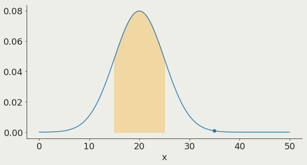
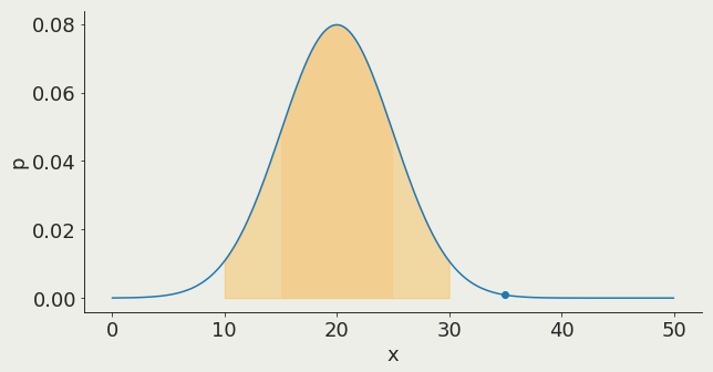
variance: n=2
standard deviation
68%
The moments of a distribution
spread (n=2)
descriptive statistics:
we summarize the proprties of a distribution
variance: n=2
standard deviation
In a Gaussian distribution:
1σ contains 68% of the distribution
68%
descriptive statistics:
we summarize the proprties of a distribution
variance: n=2
standard deviation
In a Gaussian distribution:
2σ contains 95% of the distribution
95%
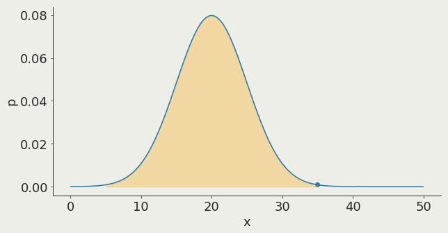
descriptive statistics:
we summarize the proprties of a distribution
variance: n=2
standard deviation
In a Gaussian distribution:
3σ contains 99.7% of the distribution
99.7%
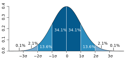
Memorize the following:
1σ = 68%
2σ = 95%
3σ = 99.7%
5σ = 99.999971428
= 1 in 3.5 million
p-value statistics
When we set a confidence value or interval on inferred quantities we imply that we had 1 in x chances of getting that result (technically "a result as extreme as that" ... we will see this in more detail
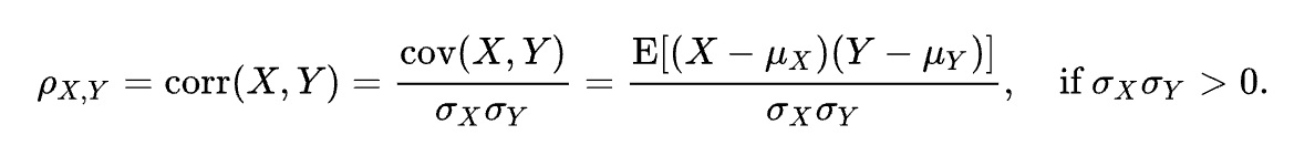
formal definition of correlation function
continuous
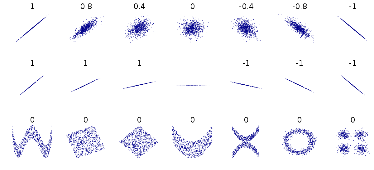
the meaning of the correlation function
The correlation function defines the degree to which a function / dataset is representative of another function / dataset
high correlation
low correlation
formal definition of correlation function
continuous
discrete
formal definition of correlation function
dot product
What does it mean?
- the integral under a curve is the area under the curve
formal definition of autocorrelation function
dot product
What does it mean?
- the dot product is larger if the points are similar
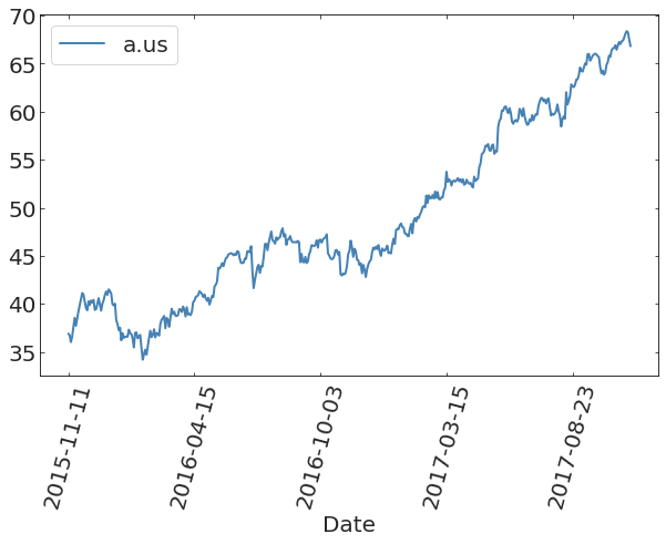
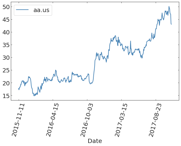
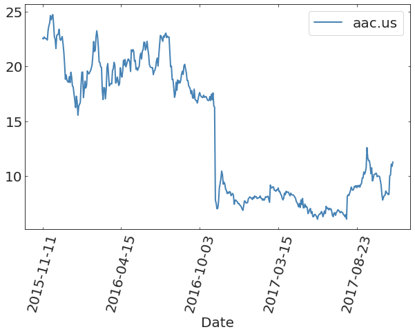
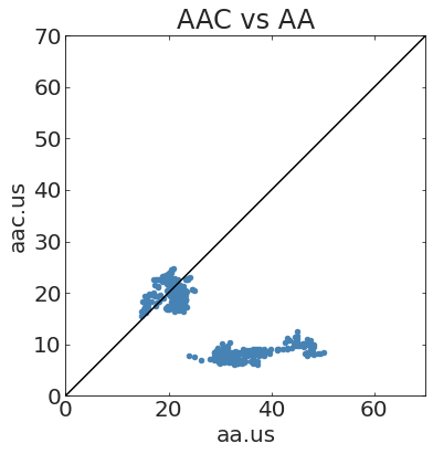
https://www.kaggle.com/datasets/borismarjanovic/price-volume-data-for-all-us-stocks-etfs/data
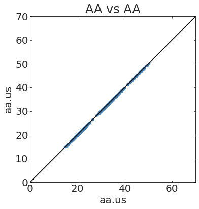
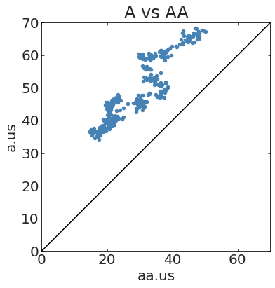
IDENTICALLY
CORRELATED
Stock Market data from Kaggle (prob HW3)
CORRELATED
NOT
CORRELATED
PEARSONS CORRELATION COEFFICIENT
(use this discussion and slides for the homework!)
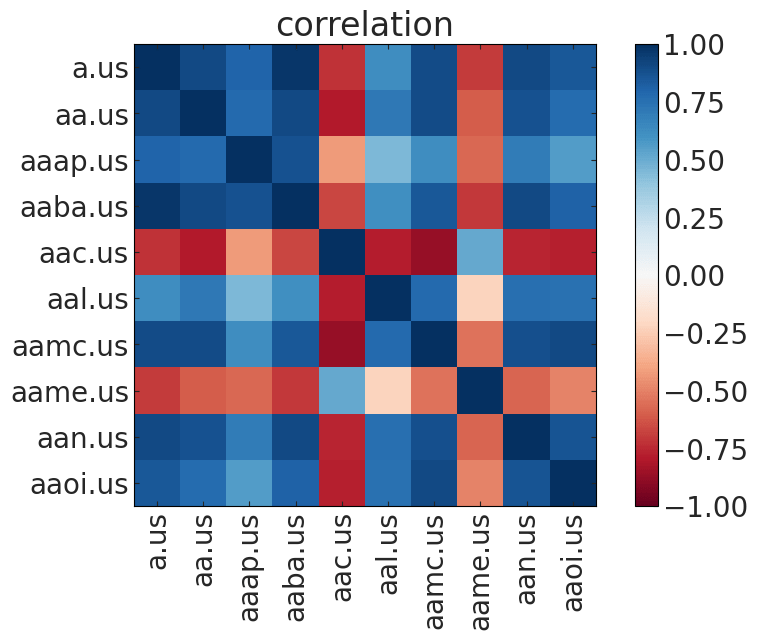
If you have many time series, you can show a "correlation matrix" that indicates the amount of correlation between each pair of time series
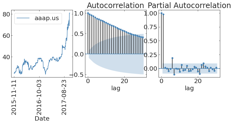
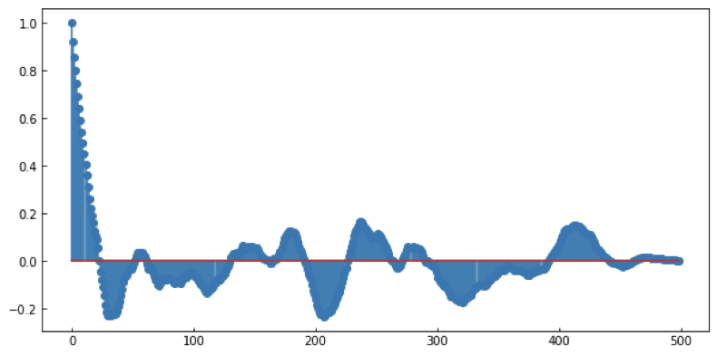
autocorrelation
2
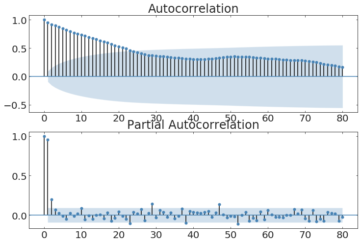
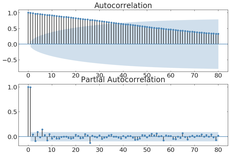
the meaning of the autocorrelation function
The autocorrelation function defines the degree to which a process has memory of itself
formal definition of autocorrelation function
is the "lag" operator
dot product
formal definition of autocorrelation function
defined for a lag j (of j steps)
formal definition of autocorrelation function
Definition
formal definition of partialautocorrelation function
Definition
autocorrelation self-similarity of the time series at a lag t
partialautocorrelation function
like ACF but controls for lag interdependence
partialautocorrelation function
like ACF but controls for lag interdependence
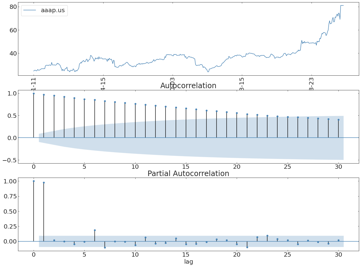
Autocorrelation and
Partial-autocorrelation
uncertainty region
(2-sigma)
anything lag falls within this region is not significant
Autocorrelation and
Partial-autocorrelation
formal definition of partialautocorrelation function
Definition
Model: a model is a mathematical formula that describes a process
it should predict some quantity (endogenous variable) from input observations (data)
it represent the way in which the endogenous variable is generated by the data
Model: a model is a mathematical formula that describes a process
it should predict some quantity (endogenous variable) from input observations (data)
it represent the way in which the endogenous variable is generated by the data
a simplification of
Model: a model is a mathematical formula that describes a process
it should predict some quantity (endogenous variable) from input observations (data)
it represent the way in which the endogenous variable is generated by the data
a simplification of
Parameter: the parameters of the model are the element of the formula which I learn from the data
Hyperparameters: what the model designer chooses before optimization
eg: the degree N of a polynomial fit (line fit N=1)
we summarize the properties of a distribution
covariance:
mean:
variance:
standard deviation:
stochastic and stationary time
processes
3
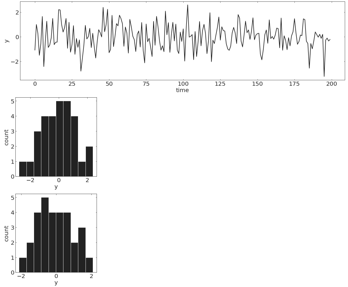
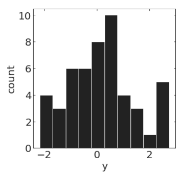
Stochastic process
A random variable indexed by time.
For any subset of points in time the dependent variable follows the a probability distribution
e.g.
pl.figure(figsize=(20,5))
N = 200
np.random.seed(100)
y = np.random.randn(N)
t = np.linspace(0, N, N, endpoint=False)
pl.plot(t, y, lw=2)
pl.xlabel("time")
pl.ylabel("y");
Discrete time stochastic process
pl.hist(y[20:70])pl.hist(y[100:150])Stochastic process
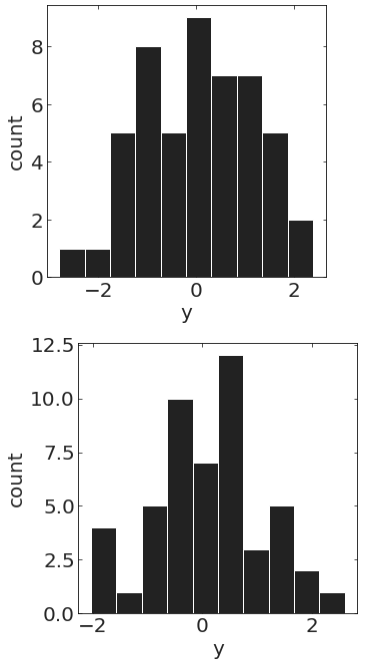
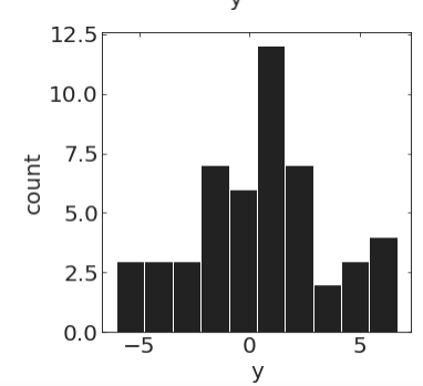
A random variable indexed by time.
For any subset of points in time the dependent variable follows the a probability distribution
e.g.
pl.figure(figsize=(20,5))
N = 200
np.random.seed(100)
y = np.random.randn(N)
t = np.linspace(0, N, N, endpoint=False)
pl.plot(t, y * t, lw=2)
pl.xlabel("time")
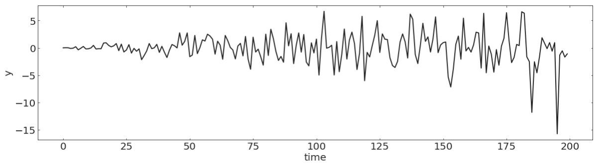
pl.ylabel("y");Discrete time stochastic process
pl.hist(y[20:70])pl.hist(y[100:150])Stochastic process
A random variable indexed by time.
Note that for the process to be stochastic the variability has to be instrinsic, not just due to noise.
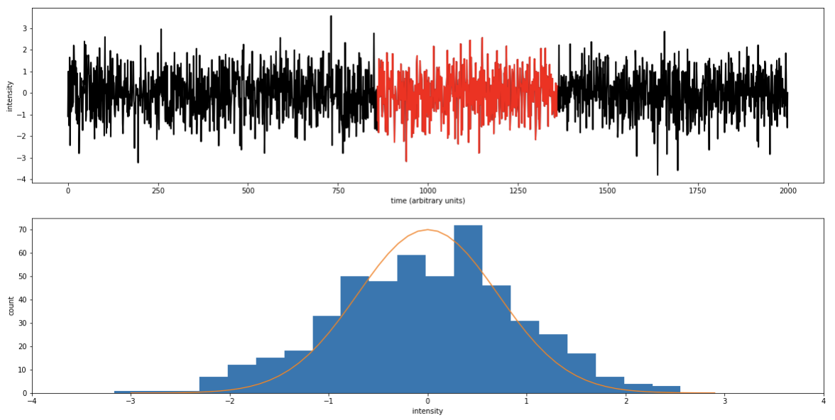
strictly stationary process
A time series is strictly stationary if for any i and Δt
strictly stationary process
A time series is strictly stationary if for any i and Δt
which implies
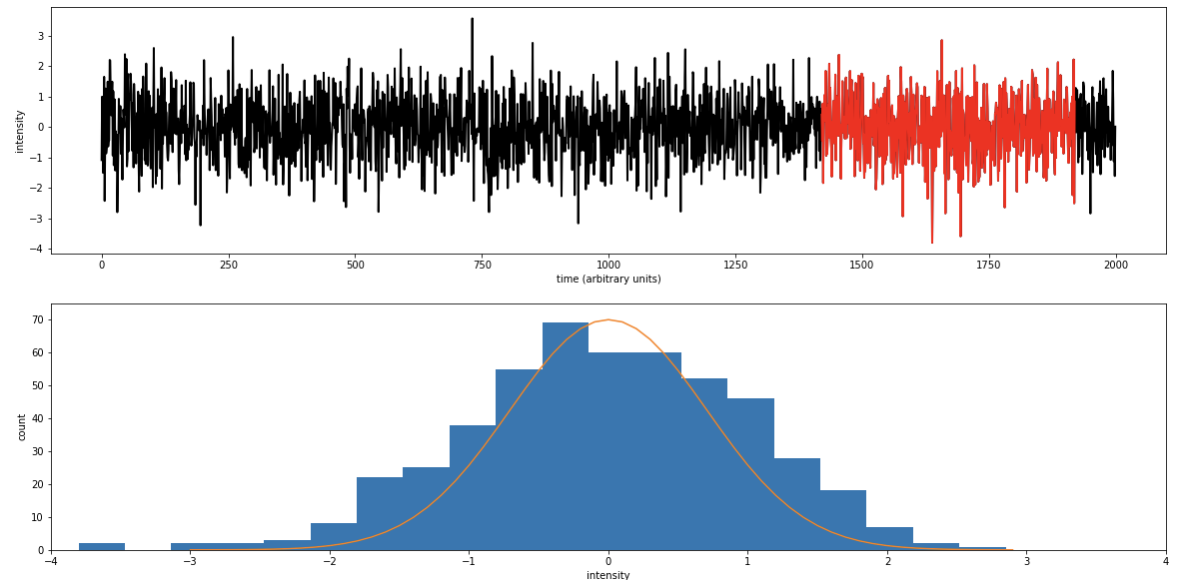
covariance stationary process
A time series is covariance stationary if for any i and Δt
Any two segments of a time series
have same mean, same variance,
same covariance
covariance stationary process
A time series is covariance stationary if for any i and Δt
The ARMA family of models
3
the AR in ARMA: AutoRegressive
The behavior at time (t) depends linearly on the behavior at time (t-1)
the AR in ARMA: AutoRegressive
The behavior at time (t) depends linearly on the behavior at time (t-1)
of course at time t I do not know the error of my prediction (ε) so the prediction is
the AR in ARMA: AutoRegressive
The behavior at time (t) depends linearly on the behavior at times (t-1)...(t-P)
coefficients
This is y = ax:
a line with slope=a and intercept = 0
the AR in ARMA: AutoRegressive
The behavior at time (t) depends linearly on the behavior at times (t-1)...(t-P)
coefficients
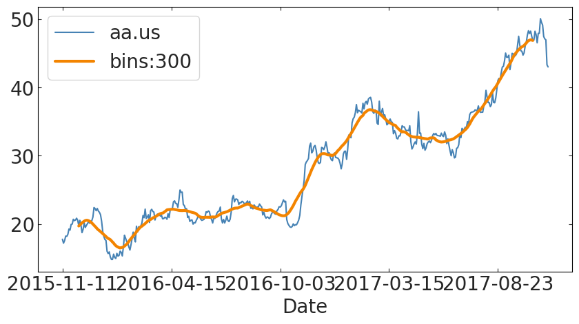
the MA in ARMA:
Moving Average
A moving average process MA(q) is a process whose current value y(t) is on average stationary and in time depends linearly on the q past values.
MA models noise around the mean.
the MA in ARMA:
Moving Average
A moving average process MA(q) is a process whose current value y(t) is on average stationary and in time depends linearly on the q past values.
MA models noise around the mean.
At time t the data value, y(t), consists of a constant, μ, plus a fraction θ (the moving-average coefficient), of the previous random noise, plus the error on this some random noise
the MA in ARMA:
Moving Average
import pylab as pl
import pandas as pd

tss["aa.us"].plot()
tss["aa.us"].rolling(30, center=True).mean().plot(
        label="bins:%d"%300, lw=3)

pl.legend();
the average of the process
some random noise cause all processes are stochastic
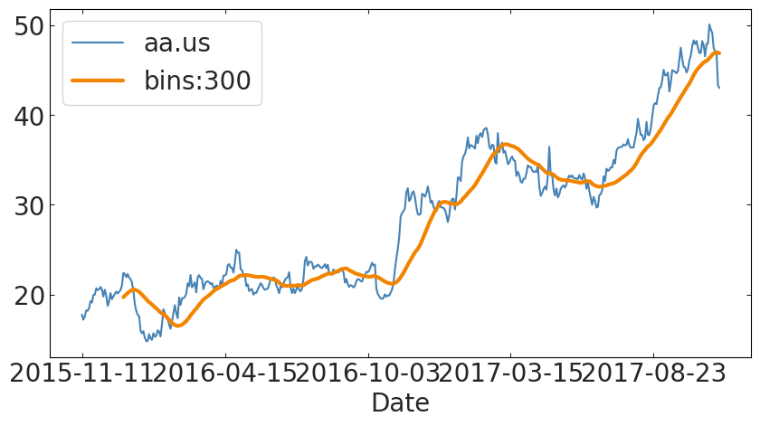
the MA in ARMA:
Moving Average
import pylab as pl
import pandas as pd

tss["aa.us"].plot()
tss["aa.us"].rolling(30, center=False).mean().plot(
        label="bins:%d"%300, lw=3)

pl.legend();
the average of the process
some random noise cause all processes are stochastic
the MA in ARMA:
Moving Average
import pylab as pl
import pandas as pd

tss["aa.us"].plot()
tss["aa.us"].rolling(30, center=False).mean().plot(
        label="bins:%d"%300, lw=3)

pl.legend();
the average of the process
some random noise cause all processes are stochastic
the MA in ARMA:
Moving Average
expect to sell on average 30 cupcakes
every day adjust based on how many cupcakes you are off:
- if you have 6 unsold, make 27 (coefficient=0.5),
- if you ran out and 2 more customers came in for a cupcake, make 31
the MA in ARMA:
Moving Average
import pylab as pl
import pandas as pd

tss["aa.us"].plot()
tss["aa.us"].rolling(30, center=False).mean().plot(
        label="bins:%d"%300, lw=3)

pl.legend();
coefficients
the MA in ARMA:
Moving Average
Note that AR(1) = MA(∞) model.
Using repeated substitution, we can demonstrate:
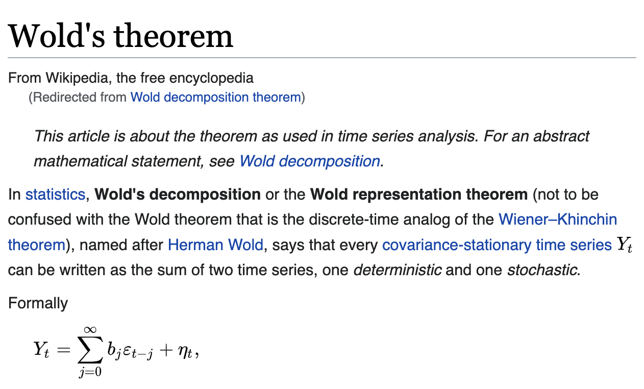
are ARMA models good?
It turns out there is a theorem that ensures that they are! BUT:
- this theorem means that if you put infinite terms the model is exact... but we put a finite number of terms in of course
- this only holds for stationary processes
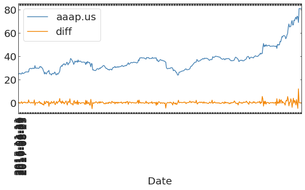
the I in ARIMA:
Integrative
I: integrative removes trends.
Turns out this model would not converge if the time series is not stationary.
ARIMA
the I in ARIMA:
Autoregressive Integrative Moving Average model
the I in ARIMA:
Autoregressive Integrative Moving Average model
p: lag order: number of lag observations in the AM model; AM(p).
q: order of the moving average: the size of the moving average window; MA(q)
d: degree of differencing: number of times that the raw observations are differenced; I(d)
Choose the What are the parameters of the model? fit for the coefficients
p ~ ?... q ~ ?
Consider the hints from the ACF and PACF as a starting point for your model design
Parameters: what is being optimized in model fitting -
eg: y = ax+b slope and intercept
ARMA coefficients
Hyperparameters: what the model designer chooses before optimization
eg: the degree N of a polynomial fit (line fit N=1)
Parameters: what is being optimized in model fitting -
eg: y = ax+b slope and intercept
ARMA coefficients
Hyperparameters: what the model designer chooses before optimization
eg: the degree N of a polynomial fit (line fit N=1)
special cases of ARIMA models
An ARIMA(0, 0, 0) model is a white noise model.
ARIMA(0, 1, 0) (or I(1) model) is a random walk.
ARIMA(0, 1, 0) with a constant is a random walk with drift.
ARIMA(0, 1, 2) is a Damped Holt's model.
ARIMA(0, 1, 1) is a basic exponential smoothing model.
An ARIMA(0, 2, 2) is equivalent to Holt's linear method with additive errors, or double exponential smoothing.
ARMA workflow
4
Model Selection
Assess if the time series is stationary
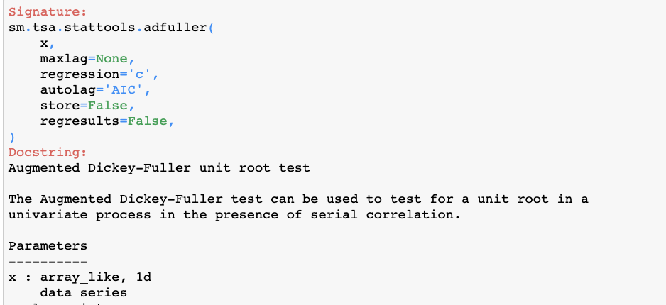
AD Fuller test:
tests the presence of a unit root
no unit root = stationary
NH: there is a unit root
AH: there is no unit root
1
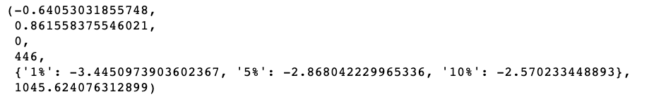
sm.tsa.stattools.adfuller(tss["aa.us"])
is stationary?
yes
no
(+)ARMA
(+)ARIMA
above threshold means cannot reject NH, i.e. there could be a unit root, i.e. it is not stationary
Model Selection
Assess if the time series is stationary
AD Fuller test:
tests the presence of a unit root
no unit root = stationary
NH: there is a unit root
AH: there is no unit root
1
sm.tsa.stattools.adfuller(tss["aa.us"])
is stationary?
yes
no
(+)ARMA
(+)ARIMA
above threshold means cannot reject NH, i.e. there could be a unit root, i.e. it is not stationary
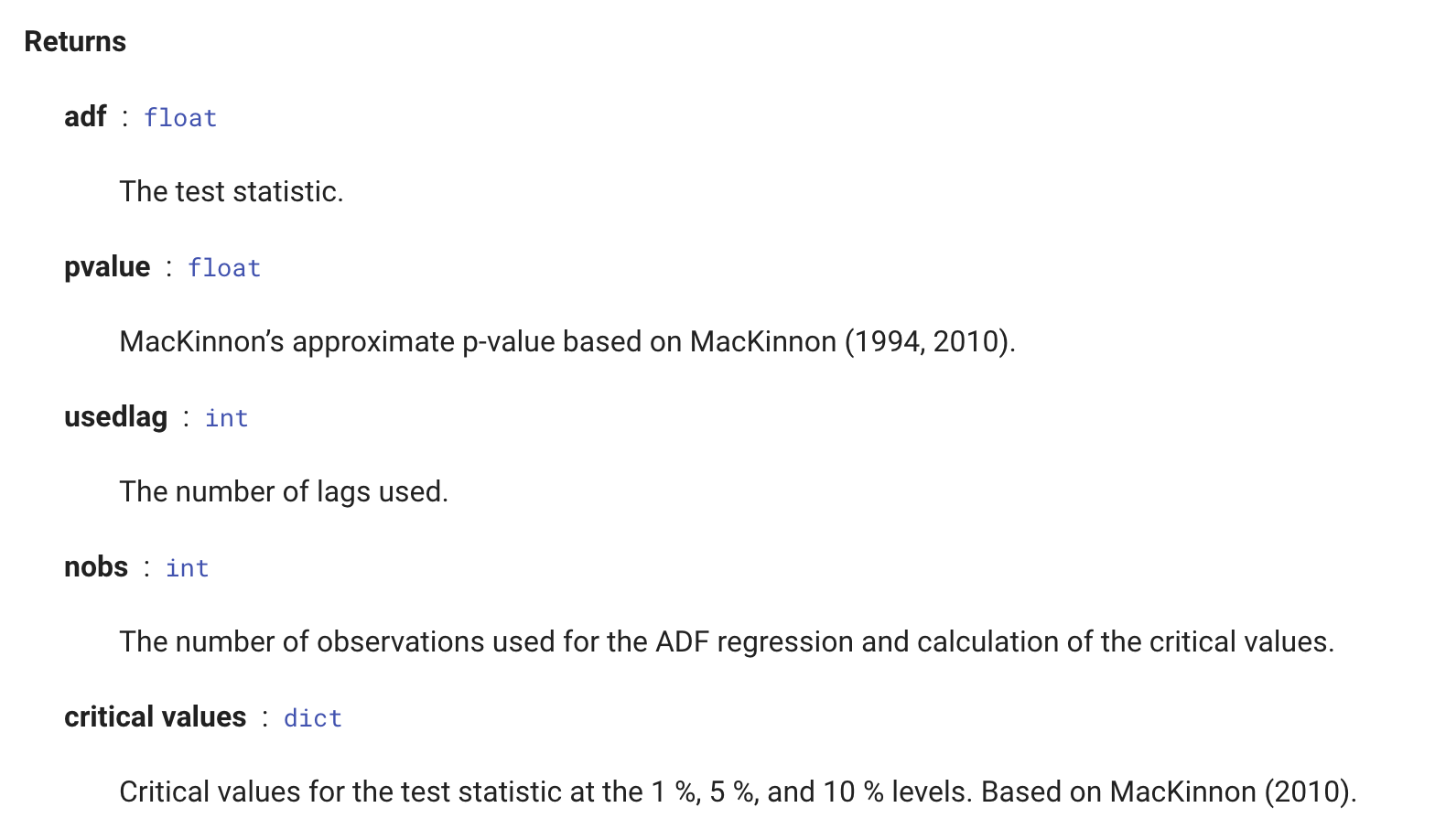
The second returned value is the p-value of the test.
Low p-values mean NH is unlikely
SET A THRESHOLD BEFORE PERFORMING THE TEST
Model Selection
Guess the "parameter" p in AR(p)- really they are hyperparameters
2
here 2 is a good guess
here maybe 1 maybe 6?
2
2 is a good guess
maybe 1 maybe 6?
Model Selection
Guess the "parameter" p in AR(p)- really they are hyperparameters
Fit models with different parameters
2
aics = np.zeros((5,5))
for p in range(5):
    for q in range(5):
            try:
                mod = sm.tsa.ARIMA(df["y"], (p,1,q)).fit()
                aics[p][q] = mod.aic
            except:
                aics[p][q] = np.nan

p,q = np.where(aic == np.nanmin(aic))
print("best parameters: p: {:d} q: {:d}".format(p[0],q[0]))
Fit model for parameters (making sure you include up to your best guess for p at least) and calculate the AIC: Aikiki Inference Criterion.
Choose the model that minimizes AIC
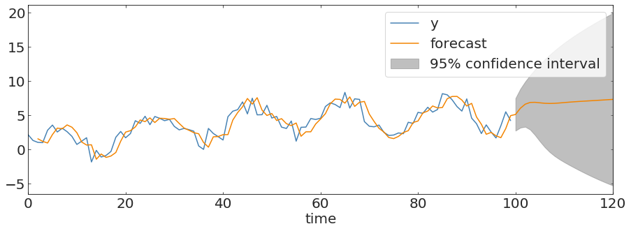
inference and forecast at last!
3
Use the model to predict or inferr
SAR(I)MA : seasonal AR(I)MA version
CAR(I)MA: works on unevenly sampled time series
VAR(I)MA: multivariate AR(I)MA
Model Selection
5
No matter what anyone tells you an answer to this question cannot be given in the abstract case: it is a domain specific question!
except:
William of Ockham (logician and Franciscan friar) 1300ca
but probably to be attributed to John Duns Scotus (1265–1308)
“Complexity needs not to be postulated without a need for it”
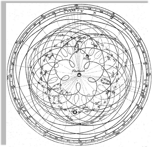
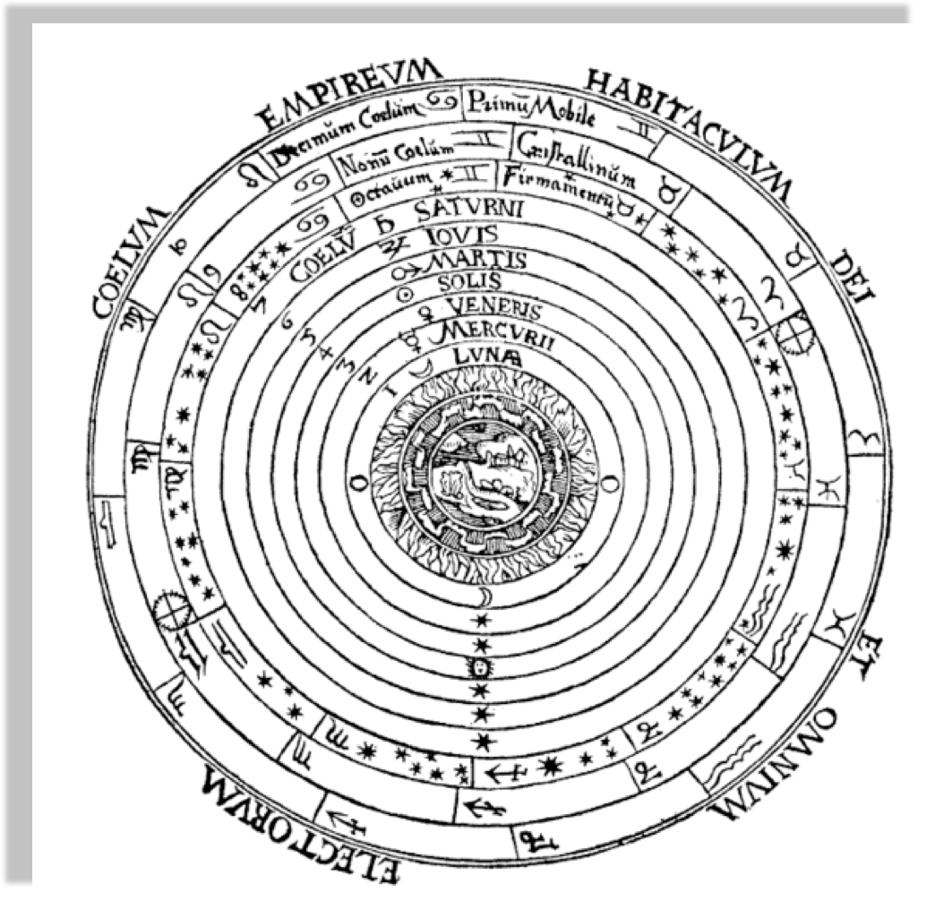
Peter Apian, Cosmographia, Antwerp, 1524 from Edward Grant,
"Celestial Orbs in the Latin Middle Ages", Isis, Vol. 78, No. 2. (Jun., 1987).
Geocentric models are intuitive:
from our perspective we see the Sun moving, while we stay still
the earth is round,
and it orbits around the sun
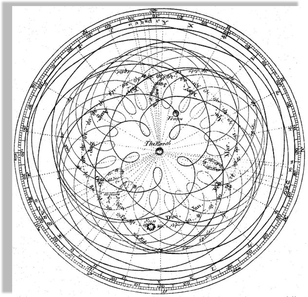
As observations improve
this model can no longer fit the data!
not easily anyways...
the earth is round,
and it orbits around the sun
Encyclopaedia Brittanica 1st Edition
Dr Long's copy of Cassini, 1777
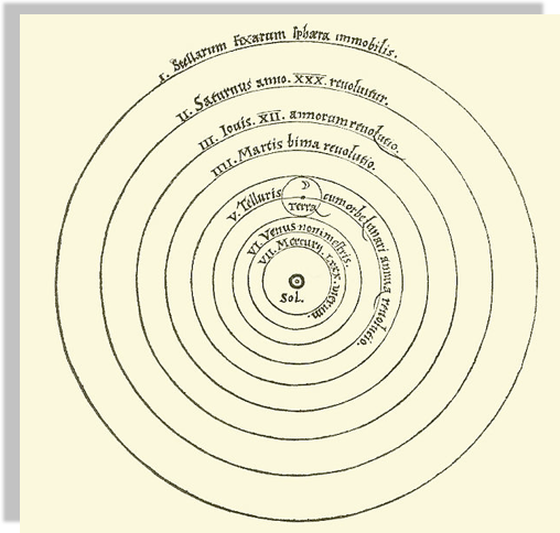
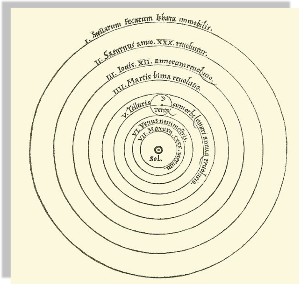
A new model that is much simpler fit the data just as well
(perhaps though only until better data comes...)
the earth is round,
and it orbits around the sun
Heliocentric model from Nicolaus Copernicus' De revolutionibus orbium coelestium.
Heliocentric model from Nicolaus Copernicus'
"De revolutionibus orbium coelestium".
Author Dr Long's copy of Cassini, 1777
Peter Apian, Cosmographia, Antwerp, 1524
Heliocentric model from Nicolaus Copernicus'
"De revolutionibus orbium coelestium".
Author Dr Long's copy of Cassini, 1777
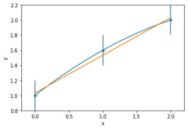
Two theories may explain a phenomenon just as well as each other. In that case you should prefer the simpler one
William of Ockham (logician and Franciscan friar) 1300ca
but probably to be attributed to John Duns Scotus (1265–1308)
“Complexity needs not to be postulated without a need for it”
“Between 2 theories that perform similarly choose the simpler one”
Between 2 theories that perform similarly choose the simpler one
In the context of model selection simpler means "with fewer parameters"
Key Concept
Since all models are wrong the scientist cannot obtain a "correct" one by excessive elaboration. On the contrary following William of Ockham he should seek an economical description of natural phenomena
Since all models are wrong the scientist must be alert to what is importantly wrong.
Science and Statistics George E. P. Box (1976)
Journal of the American Statistical Association, Vol. 71, No. 356, pp. 791-799.
No matter what anyone says an answer to this question cannot be given in the abstract case: it is a domain specific question!
except:
the case of ARIMA models
Ockham’s razor: Pluralitas non est ponenda sine neccesitate
or “the law of parsimony”
William of Ockham (logician and Franciscan friar) 1300ca
but probably to be attributed to John Duns Scotus (1265–1308)
”Complexity needs not to be postulated without a need for it”
“Between 2 theories choose the simpler one”
“Between 2 theories choose the one with fewer parameters"
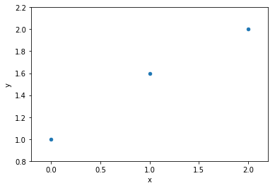
data
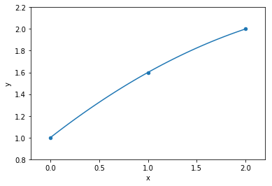
model fit to data
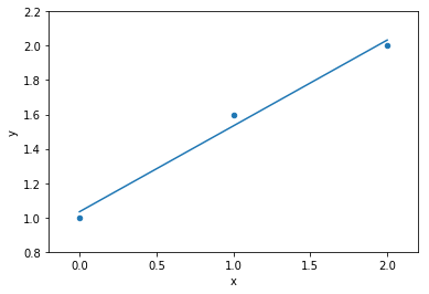
model fit to data
model fit to data
1 variable: x
model fit to data
parameters
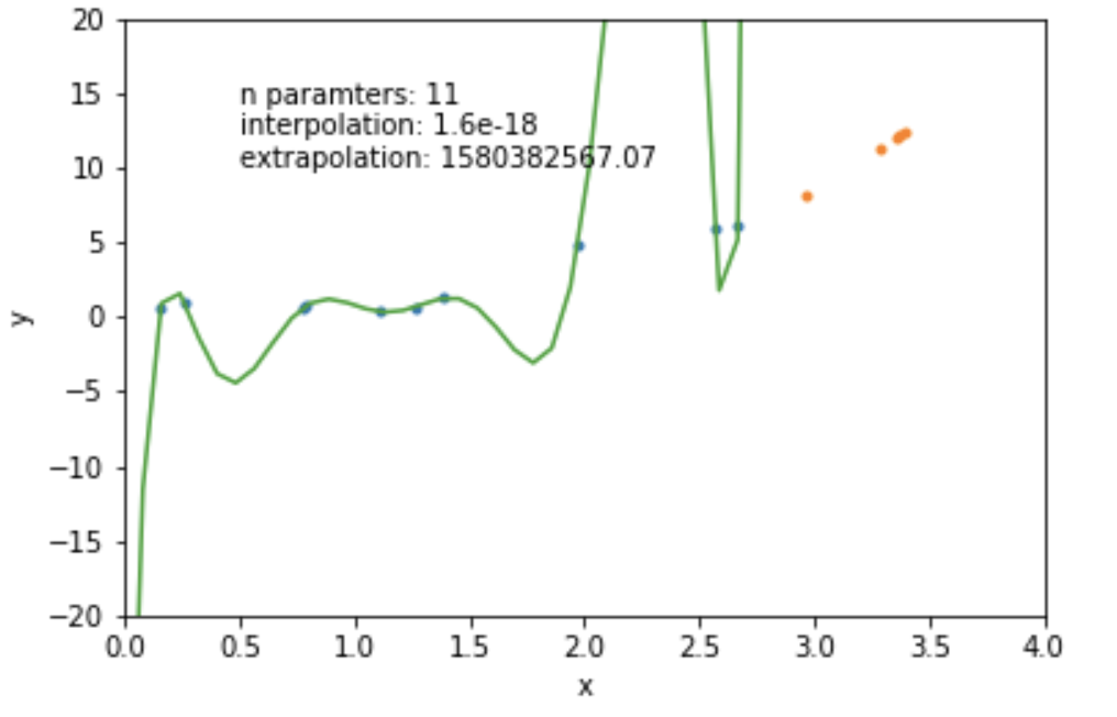
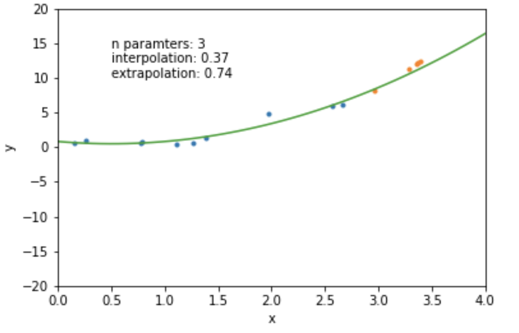
the complexity of a model can be measured by the number of variables and the numbers of parameters
the complexity of a model can be measured by the number of variables and the numbers of parameters
mathematically: given N data points there exist an N-features model that goes exactly through each data point. but is it useul??
Overfitting: fitting data with a model that is too complex and that does not extend to new data (low predictive power on test data)
Model Diagnostics
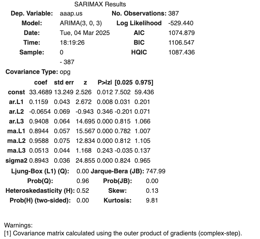
model = sm.tsa.ARIMA(endog = train_set, order=(3,
iorder, 3)).fit()Akaike information criterion (AIC) .
L is the likelihood of the data, p is the order of the autoregressive part and q is the order of the moving average part. The k represents the intercept of the ARIMA model.
AIC can only be used to compare ARIMA models with the same orders of differencing. For ARIMAs with different orders of differencing, RMSE can be used for model comparison.
Choose model (hyper)-parameters that minimize AIC
Akaike information criterion (AIC) .
The preferred ARIMA models among a family of models with the same orders of differencing is the one that minimized the Aikiki Imformation Criterion (AIC).
Key Concept
Bayes Theorem &
Bayesian statistics
6
posterior
likelihood
prior
evidence
model parameters
data
D
constraints on the model
e.g. flux is never negative
P(f<0) = 0 P(f>=0) = 1
prior:
model parameters
data
D
constraints on the model
e.g. flux is never negative
P(f<0) = 0 P(f>=0) = 1
prior:
model parameters
data
D
model parameters
data
D
model parameters
data
D
model parameters
data
D
prior:
constraints on the model
people's weight <1000lb
& people's weight >0lb
P(w) ~ N(105lb, 90lb)
model parameters
data
D
prior:
constraints on the model
people's weight <1000lb
& people's weight >0lb
P(w) ~ N(105lb, 90lb)
the prior should not be 0 anywhere the probability might exist
model parameters
data
D
prior:
"uninformative prior"
likelihood:
this is our model
model parameters
data
D
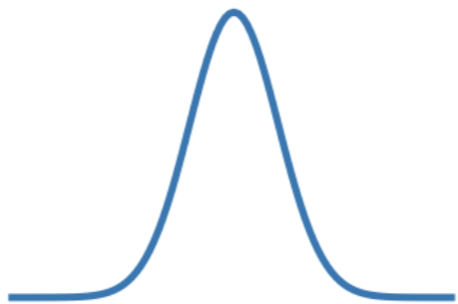
evidence
????
model parameters
data
D
evidence
????
model parameters
data
D
it does not matter if I want to use this for model comparison
model parameters
data
D
it does not matter if I want to use this for model comparison
which has the highest posterior probability?
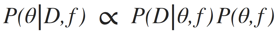
posterior: joint probability distributin of a parameter set (θ, e.g. (m, b)) condition upon some data D and a model hypothesys f
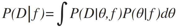
evidence: marginal likelihood of data under the model
prior: “intellectual” knowledge about the model parameters condition on a model hypothesys f. This should come from domain knowledge or knowledge of data that is not the dataset under examination
posterior: joint probability distributin of a parameter set (θ, e.g. (m, b)) condition upon some data D and a model hypothesys f
evidence: marginal likelihood of data under the model
prior: “intellectual” knowledge about the model parameters condition on a model hypothesys f. This should come from domain knowledge or knowledge of data that is not the dataset under examination
in reality all of these quantities are conditioned on the shape of the model: this is a model fitting, not a model selection methodology
model selection methodology
AIC BIC MLD
7
Shannon 1948: A Mathematical Theory of Communication
a theory to find fundamental limits on signal processing and communication operations such as data compression
model selection is also based on the minimization of a quantity. Several quantities are suitable:
MLD
BIC
Bayese theorem
AIC
Optimism and likelihood maximization on the training set
Akaike information criterion (AIC) .
Based on
where is a family of function (=densities) containing the correct (=true) function and is the set of parameters that maximized the likelihood L
L is the likelihood of the data, k is the number of parameters,
N the number of variables.
number of parameters:
Model Complexity
Likelihood: Model Performance.
"-" sign in front of the log-likelihood: AIC shrinks for better models,
AIC ~ k => is linearly proportional to (grows with) the number of parameters
Likelihood: Model Performance.
number of parameters:
Model Complexity
Bayesian information criterion (BIC) .
L is the likelihood of the data, k is the number of parameters,
N the number of variables.
stronger penalization of complexity (as long as N> )
The derivation is very different:
Bayes Factor
Minimum Description Length (MDL) .
negative log-likelihood of the model parameters (θ) and the negative log-likelihood of the target values (y) given the input values (X) and the model parameters (θ).
also: log(L(θ)): number of bits required to represent the model,
log(L(y| X,θ)): number of bits required to represent the predictions on observations
minimize the encoding of the model and its predictions
derived from Shannon's theorem of information
Mathematically similar, though derived from different approaches. All used the same way: the preferred model is the model that minimized the estimator
Model Optimization
with MCMC
8
stochastic
"markovian"
sequence
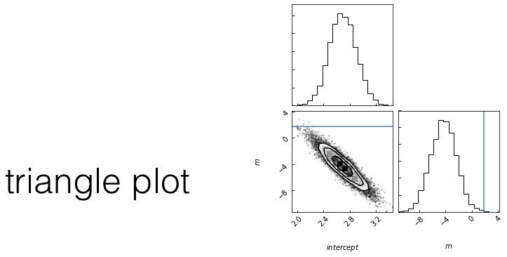
posterior: joint probability distributin of a parameter set (m, b) conditioned upon some data D and a model hypothesys f
Goal: sample the posterior distribution
slope
intercept
slope
Goal: sample the posterior distribution
choose a starting point in the parameter space: current = θ0 = (m0,b0)
WHILE convergence criterion is met:
calculate the current posterior pcurr = P(D|θ0,f)
//proposal
choose a new set of parameters new = θnew = (mnew,bnew)
calculate the proposed posterior pnew = P(D|θnew,f)
IF pnew/pcurr < 1:
current = new
ELSE:
//probabilistic step: accept with probability pnew/pcurr
draw a random number r ૯U[0,1]
IF r > pnew/pcurr >:
current = new
ELSE:
pass // do nothing
stochasticity allows us to explore the whole surface but spend more time in interesting spots
Goal: sample the posterior distribution
choose a starting point in the parameter space: current = θ0 = (m0,b0)
WHILE convergence criterion is met:
calculate the current posterior pcurr = P(D|θ0,f)
//proposal
choose a new set of parameters new = θnew = (mnew,bnew)
calculate the proposed posterior pnew = P(D|θnew,f)
IF pnew/pcurr > 1:
current = new
ELSE:
Questions:
1. how do I choose the next point?
Any Markovian ergodic process
choose a starting point in the parameter space: current = θ0 = (m0,b0)
WHILE convergence criterion is met:
calculate the current posterior pcurr = P(D|θ0,f)
//proposal
choose a new set of parameters new = θnew = (mnew,bnew)
calculate the proposed posterior pnew = P(D|θnew,f)
IF pnew/pcurr > 1:
current = new
ELSE:
//probabilistic step: accept with probability pnew/pcurr
draw a random number r ૯U[0,1]
IF r > pnew/pcurr >:
current = new
ELSE:
pass // do nothing
A process is Markovian if the next state of the system is determined stochastically as a perturbation of the current state of the system, and only the current state of the system, i.e. the system has no memory of earlier states (a memory-less process).
(given enough time) the entire parameter space would be sampled.
At equilibrium, each elementary process should be equilibrated by its reverse process.
reversible Markov process
Detailed Balance is a sufficient condition for ergodicity
Metropolis Rosenbluth Rosenbluth Teller 1953 - Hastings 1970
If the chains are a Markovian Ergodic process
the algorithm is guaranteed to explore the entire likelihood surface given infinite time
This is in contrast to gradient descent, which can get stuck in local minima or in local saddle points.
how to choose the next point
how you make this decision names the algorithm
simulated annealing (good for multimodal)
parallel tempering (good for multimodal)
differential evolution (good for covariant spaces)
Gibbs sampling (move in along one variable at a time)
choose a starting point in the parameter space: current = θ0 = (m0,b0)
WHILE convergence criterion is met:
calculate the current posterior pcurr = P(D|θ0,f)
//proposal
choose a new set of parameters new = θnew = (mnew,bnew)
calculate the proposed posterior pnew = P(D|θnew,f)
IF pnew/pcurr > 1:
current = new
ELSE:
//probabilistic step: accept with probability pnew/pcurr
draw a random number r ૯U[0,1]
IF r > pnew/pcurr >:
current = new
ELSE:
pass // do nothing
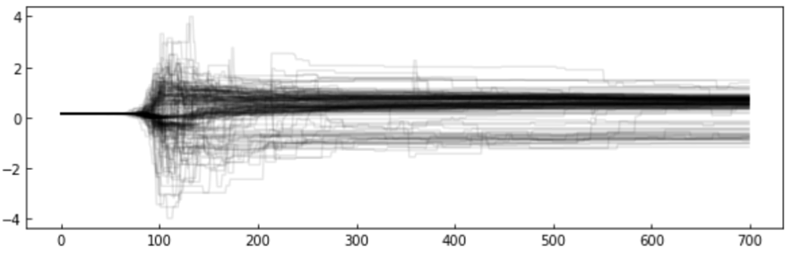
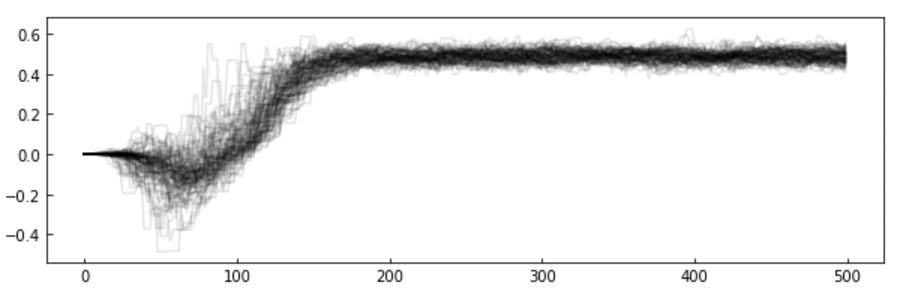
The chains: the algorithm creates a "chain" (a random walk) that "explores" the likelihood surface.
More efficient is to run many parallel chains - each exploring the surface, an "ensemble"
The path of the chains can be shown along each feature
choose a starting point in the parameter space: current = θ0 = (m0,b0)
WHILE convergence criterion is met:
calculate the current posterior pcurr = P(D|θ0,f)
//proposal
choose a new set of parameters new = θnew = (mnew,bnew)
calculate the proposed posterior pnew = P(D|θnew,f)
IF pnew/pcurr > 1:
current = new
ELSE:
//probabilistic step: accept with probability pnew/pcurr
draw a random number r ૯U[0,1]
IF r > pnew/pcurr >:
current = new
ELSE:
pass // do nothing
step
feature value
Examples of how to choose the next point
affine invariant : EMCEE package
choose a starting point in the parameter space: current = θ0 = (m0,b0)
WHILE convergence criterion is met:
calculate the current posterior pcurr = P(D|θ0,f)
//proposal
choose a new set of parameters new = θnew = (mnew,bnew)
calculate the proposed posterior pnew = P(D|θnew,f)
IF pnew/pcurr > 1:
current = new
ELSE:
//probabilistic step: accept with probability pnew/pcurr
draw a random number r ૯U[0,1]
IF r > pnew/pcurr >:
current = new
ELSE:
pass // do nothing
step
feature value
MCMC convergence
MCMC convergence
MCMC convergence
MCMC convergence
MCMC convergence
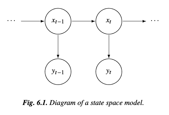
State Space Model
4.1
motion equations for the position or "state" of a spacecraft
x(t): location
y(t): information that can be observed from a tracking device such as velocity and azimuth
unobserved state
Underlying state x is a time varying Markovian process (the position of the pace craft)
The observed variable depends at least on the state and on noise.
Other elements (e.g. seasonality) can be included in the model too
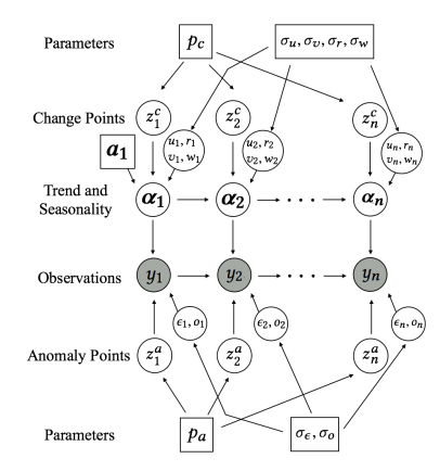
we can write a Bayesian structural model like this:
local level
state
seasonal trend
we can write a Bayesian structural model like this:
seasonal variations
unobserved trend
Its a Markovian Process:
stochastic process with 1-step memory
there is a hidden or latent process xt called the state process (the position of the space craft)
a bit more complex
A model that accepts regression on exogenous variables allows feature extraction: which features are important in the prediction?
e.g. CO2 or Irradiance in climate change (HW)
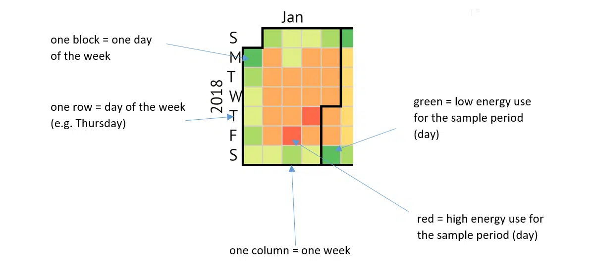
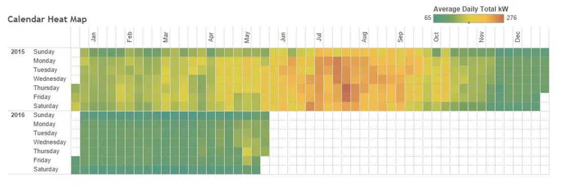
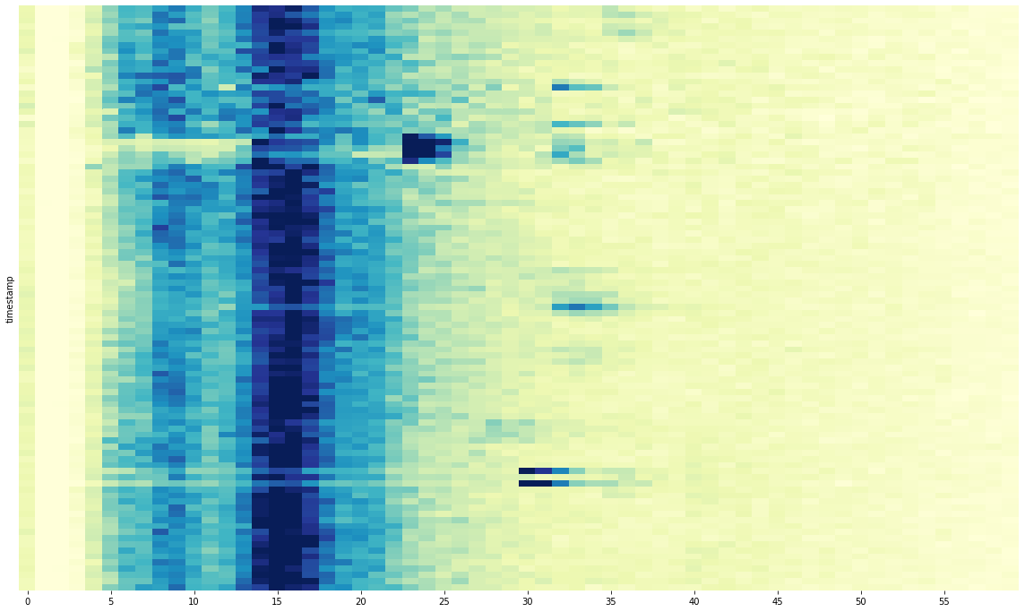
The essence of the calendar heat map is viewing data over at a glance. Imagine a calendar, tipped on its side so the days of the week run vertically:
sns.heatmap(minutely, robust=True, cmap='YlGnBu',
            yticklabels=False, xticklabels=5, cbar=False)
https://jonisalonen.com/2019/plotting-a-time-series-heat-map-with-pandas/
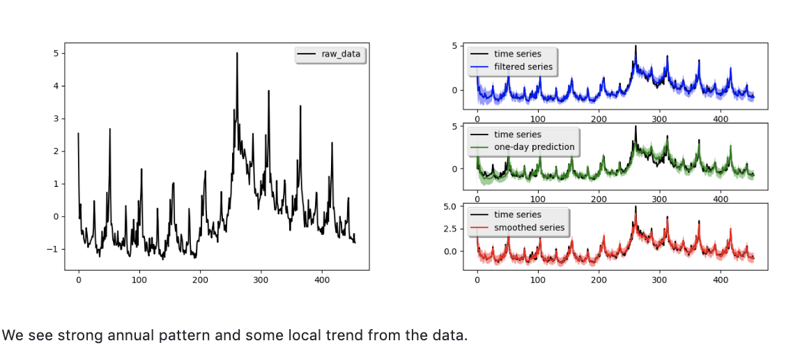
Sorry ARIMA, but I’m Going Bayesian
https://multithreaded.stitchfix.com/blog/2016/04/21/forget-arima/
Sorry ARIMA, but I’m Going Bayesian
https://multithreaded.stitchfix.com/blog/2016/04/21/forget-arima/
Elements of Statistical Learning Chapter 7
https://towardsdatascience.com/implementing-facebook-prophet-efficiently-c241305405a3
By federica bianco
Autoregressive models, model selection, Bayes theorem


