


federica bianco PRO
astro | data science | data for good
Anomaly Detection and Point of Change Analysis
Fall 2025 - UDel PHYS 661
dr. federica bianco
@fedhere
this slide deck:
LR = _____________________________
True Negative
False Negative
| H0 is True | H0 is False | |
|---|---|---|
| H0 is falsified | Type I Error False Positive |
True Positive |
|
H0 is not falsified |
True Negative | Type II Error False Negative |
LR = _____________________________
True Negative
False Negative
| H0 is True | H0 is False | |
|---|---|---|
| H0 is falsified | Type I Error False Positive |
True Positive |
|
H0 is not falsified |
True Negative | Type II Error False Negative |
important message spammed
spam in
your inbox
Anomaly detection
1
What is an outlier?
What is an outlier?
for now we'll focus on outlier events in time series: anomalies
literally it lies outside of the distribution.
The only problem is that generally I do now know what the distribution is....
What is an outlier?
literally it lies outside of the distribution.
The only problem is that generally I do now know what the distribution is....
generally I will assume that points that are "far" from the "core" of the distribution are outliers, but this definition betrays I have some belief about the distribution itself
What is an outlier?
point-wise detection (time points as outliers)
pattern-wise detection (subsequences as outliers)
system-wise detection (time series as outliers).
What is an outlier?
remember the definition of stochastic:
P(t) = P(t+l) for any l lag
Anomaly in a stochastic process
remember the definition of stochastic:
P(t) = P(t+l) for any l lag
if you believe you have a good model you can choose a frequentist approach and define a threshold corresponding to a p-value
Anomaly in a stochastic process
remember the definition of stochastic:
P(t) = P(t+l) for any l lag
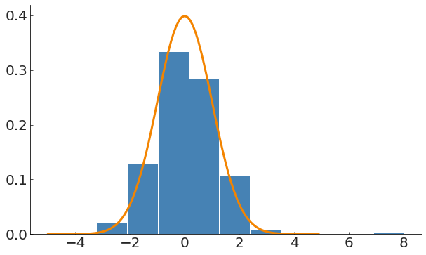
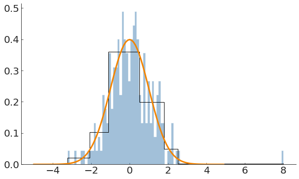
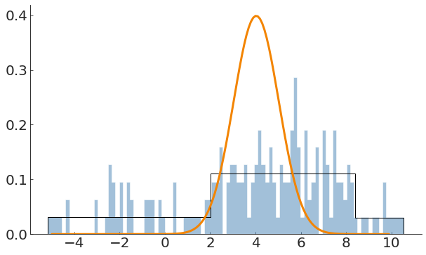
Note also that a lot of your inference will depend on how you generate a distribution from your data: what is the right number of bins in a histogram?
If the distribution is not stochastic I recommend you look at adaptive binning, e.g. Bayesian Blocks
https://arxiv.org/pdf/1207.5578.pdf
This is an ideal framework for anomaly detection in time series where the time of arrival is the variable recorded
Anomaly in a stochastic process
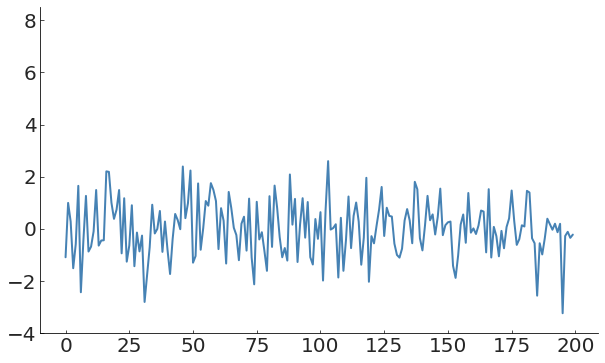
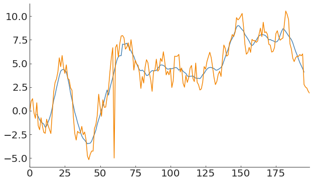
what if you do not have a good model? what if the generative process is time dependent?
Anomaly in a time-varying process
what if you do not have a good model? what if the generative process is time dependent?
Anomaly in a time-varying process
A global measure of the process does not capture anomalies in time-evolving processes
pl.plot(x, y)
m = y.mean()
s = y.std()
pl.plot(x, m, lw=3)
pl.plot(x, m + 3 * s, c='k')
pl.plot(x, m - 3 * s, c='k')
Anomaly in a time-varying process
simple detection methods
2.1
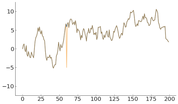
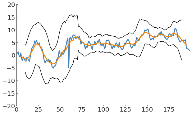
what if you do not have a good model? what if the generative process is time dependent?
m = df['y'].rolling(window=10, center=True).mean()
df['y'].plot(lw=3)
df['m'].plot(lw=3)
(m + 3 * df['y'].rolling(window=20, center=True).std()).plot(c='k')
(m - 3 * df['y'].rolling(window=20, center=True).std()).plot(c='k')
in this case its still not enough!
Anomaly in a time-varying process
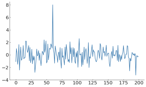
what if you do not have a good model? what if the generative process is time dependent?
Anomaly in a time-varying process
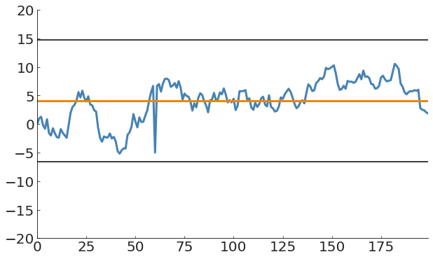
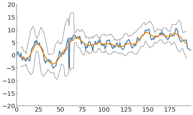
m = df['y'].rolling(window=11,
center=True).apply(lambda x:
np.mean(np.concatenate([x[:5], x[6:]])))
s = df['y'].rolling(window=11,
center=True).apply(lambda x:
np.std(np.concatenate([x[:5], x[6:]])))
(m + 3 * s).plot(c='k', alpha=0.5)
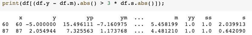
(m - 3 * s).plot(c='k', alpha=0.5)This works well for single point anomalies
what if you do not have a good model? what if the generative process is time dependent?
Anomaly in a time-varying process
This works well for single point anomalies
Remember that at 3-sigma you expect 3 detections in 1000 measurements
Bayesian outliers detection
2.2
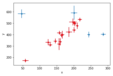
Simple case: we believe our generative process is a line
y=mx+b
and some additive noise
e~N(μ,σ)
def lnlike(theta, x, y, yerr):
    m, b, Yb = theta
    #line fit model
    model = m * x + b
    #variance of data
    sig2 = yerr**2
     #normalization: this is importnat because we have 2 linearly combined pieces of model
    den = 2 * np.pi * sig2
    #this is the probability that the point comes from the line
    a = 1 / np.sqrt(den) *\
        exp(-(y-model)**2 /  2.0 / sig2)
return np.sum(np.log(a))Simple case: we believe our generative process is a line
y=mx+b
and some additive noise
e~N(μ,σ)
def lnprior(theta):
    '''
    logprior on the parameters theta
    theta: 5 parameter vector: slpoe, intercept
    '''
    m, b = theta
    if -200 < b < 500 and 0 < m < 10.0 :
        return 0.0
    return -np.inf
def lnprob(theta, x, y, yerr):
    ''' log likelihood * log prior: the posterior
    '''
    lp = lnprior(theta)

    if not np.isfinite(lp) :
        return -np.inf
    lnl = lnlike(theta, x, y, yerr)
    if  np.isnan(lnl):
        return -np.inf
return lp + lnl Simple model: we believe our generative process is a line
y=mx+b
and some additive noise
e~N(μ,σ)
Upgrade: we believe our generative process is a line
y=mx+b
and some additive noise
e~N(μ,σ)
plus another Gaussian process that can generate some points
Fitting a straight line to data,
https://arxiv.org/pdf/1008.4686.pdf
Hogg, Bovy, Lang 2010,
Section 3, Pruning outliers
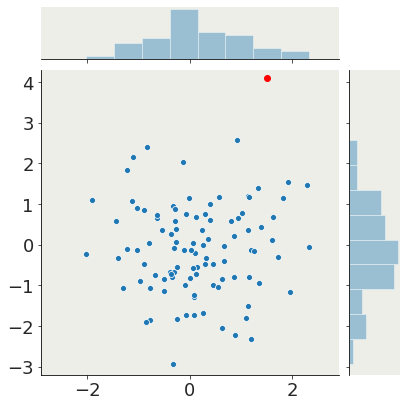
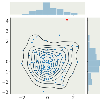
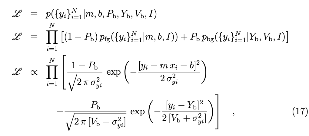
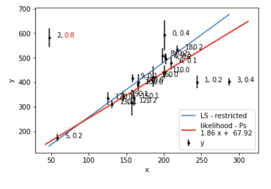
in the presence of more than one generative process, one which generates inliers one that generates outliers, each point has a probability of being generated by either process!
Key Concept
Upgrade: we believe our generative process is a line
y=mx+b
and some additive noise
e~N(μ,σ)
plus another Gaussian process that can generate some points
def lnlike(theta, x, y, yerr):
    m, b, Yb, Pb, V = theta
    #line fit model
    model = m * x + b
    #variance of data
    sig2 = yerr**2
     #normalization: this is importnat because
     #we have 2 linearly combined pieces of model
    den = 2 * np.pi * sig2
    #this is the probability that the point comes from the line
    a = (1 - Pb) / np.sqrt(den) *\
        exp(-(y-model)**2 /  2.0 / sig2)
    #this is the probability that it does not
    b = Pb / np.sqrt(den + 2*np.pi*V) *\
        exp (-(y - Yb)**2 / 2 / (V + sig2))
    return  np.sum(np.log(a + b))
Pb probability of outlier
pfg, probability distribution of the foreground model (inliers)
pbg probability distribution of the background model (outliers)
Upgrade: we believe our generative process is a line
y=mx+b
and some additive noise
e~N(μ,σ)
plus another Gaussian process that can generate some points
def lnlike(theta, x, y, yerr):
    m, b, Yb, Pb, V = theta
    #line fit model
    model = m * x + b
    #variance of data
    sig2 = yerr**2
     #normalization: this is importnat because we have 2 linearly combined pieces of model
    den = 2 * np.pi * sig2
    #this is the probability that the point comes from the line
    a = (1 - Pb) / np.sqrt(den) *\
        exp(-(y-model)**2 /  2.0 / sig2)
    #this is the probability that it does not
    b = Pb / np.sqrt(den + 2*np.pi*V) *\
        exp (-(y - Yb)**2 / 2 / (V + sig2))
    return  np.sum(np.log(a + b))
def lnprior(theta):
'''
logprior on the parameters theta
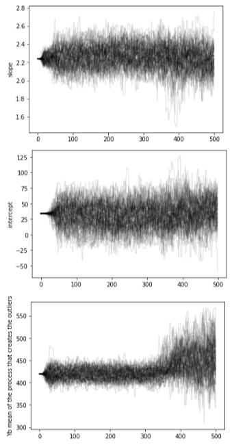
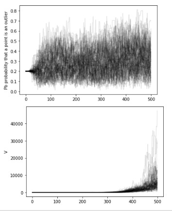
theta: 5 parameter vector: slpoe, intercept,
Yb mean of the process that creates the outliers,
Pb probability that a point is an outlier,
V the variance of the process that generates outliers
'''
m, b, Yb, Pb, V = theta
if -200 < b < 500 and 0 < m < 10.0 :
#Pb is a probability so it is bound to 0-1
if Pb < 0 or Pb > 1:
return -np.inf
# set some constraints on the mean of the process that creates the outliers
if Yb > ymean + 150 or Yb < ymean - 150:
return -np.inf
if V < 0:
return -np.inf
#print("3")
return 0.0
return -np.inf
def lnprob(theta, x, y, yerr):
''' log likelihood * log prior: the posterior
'''
lp = lnprior(theta)
if not np.isfinite(lp) :
return -np.inf
lnl = lnlike(theta, x, y, yerr)
if np.isnan(lnl):
return -np.inf
return lp + lnl Upgrade: we believe our generative process is a line
y=mx+b
and some additive noise
e~N(μ,σ)
plus another Gaussian process that can generate some points
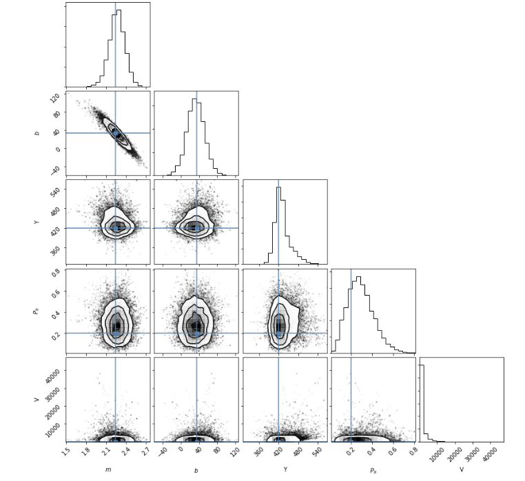
new model parameters
simple model parameters
Upgrade: we believe our generative process is a line
y=mx+b
and some additive noise
e~N(μ,σ)
plus another Gaussian process that can generate some points
Getting the probability that each point is an outlier
(exercise!)
stochastic
"markovian"
sequence
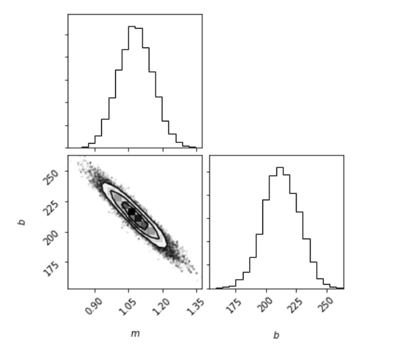
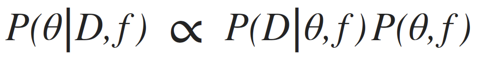
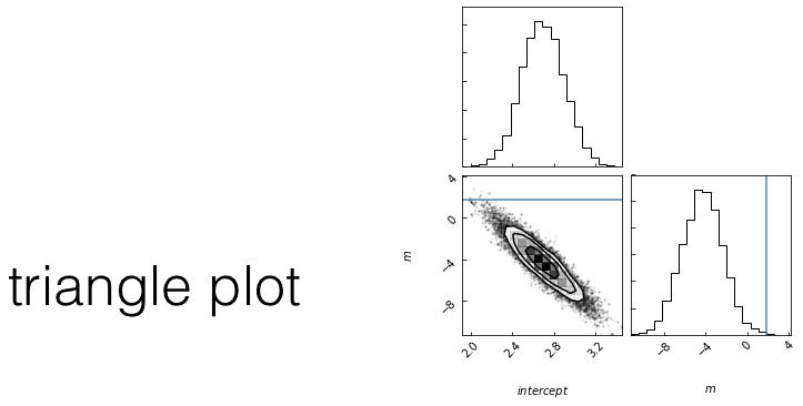
posterior: joint probability distributin of a parameter set (m, b) conditioned upon some data D and a model hypothesys f
Goal: sample the posterior distribution
slope
intercept
slope
Goal: sample the posterior distribution
choose a starting point in the parameter space: current = θ0 = (m0,b0)
WHILE convergence criterion is met:
calculate the current posterior pcurr = P(D|θ0,f)
//proposal
choose a new set of parameters new = θnew = (mnew,bnew)
calculate the proposed posterior pnew = P(D|θnew,f)
IF pnew/pcurr < 1:
current = new
ELSE:
//probabilistic step: accept with probability pnew/pcurr
draw a random number r ૯U[0,1]
IF r > pnew/pcurr >:
current = new
ELSE:
pass // do nothing
stochasticity allows us to explore the whole surface but spend more time in interesting spots
Goal: sample the posterior distribution
choose a starting point in the parameter space: current = θ0 = (m0,b0)
WHILE convergence criterion is met:
calculate the current posterior pcurr = P(D|θ0,f)
//proposal
choose a new set of parameters new = θnew = (mnew,bnew)
calculate the proposed posterior pnew = P(D|θnew,f)
IF pnew/pcurr > 1:
current = new
ELSE:
Questions:
1. how do I choose the next point?
Any Markovian ergodic process
choose a starting point in the parameter space: current = θ0 = (m0,b0)
WHILE convergence criterion is met:
calculate the current posterior pcurr = P(D|θ0,f)
//proposal
choose a new set of parameters new = θnew = (mnew,bnew)
calculate the proposed posterior pnew = P(D|θnew,f)
IF pnew/pcurr > 1:
current = new
ELSE:
//probabilistic step: accept with probability pnew/pcurr
draw a random number r ૯U[0,1]
IF r > pnew/pcurr >:
current = new
ELSE:
pass // do nothing
A process is Markovian if the next state of the system is determined stochastically as a perturbation of the current state of the system, and only the current state of the system, i.e. the system has no memory of earlier states (a memory-less process).
(given enough time) the entire parameter space would be sampled.
At equilibrium, each elementary process should be equilibrated by its reverse process.
reversible Markov process
Detailed Balance is a sufficient condition for ergodicity
Metropolis Rosenbluth Rosenbluth Teller 1953 - Hastings 1970
If the chains are a Markovian Ergodic process
the algorithm is guaranteed to explore the entire likelihood surface given infinite time
This is in contrast to gradient descent, which can get stuck in local minima or in local saddle points.
how to choose the next point
how you make this decision names the algorithm
simulated annealing (good for multimodal)
parallel tempering (good for multimodal)
differential evolution (good for covariant spaces)
Gibbs sampling (move in along one variable at a time)
choose a starting point in the parameter space: current = θ0 = (m0,b0)
WHILE convergence criterion is met:
calculate the current posterior pcurr = P(D|θ0,f)
//proposal
choose a new set of parameters new = θnew = (mnew,bnew)
calculate the proposed posterior pnew = P(D|θnew,f)
IF pnew/pcurr > 1:
current = new
ELSE:
//probabilistic step: accept with probability pnew/pcurr
draw a random number r ૯U[0,1]
IF r > pnew/pcurr >:
current = new
ELSE:
pass // do nothing
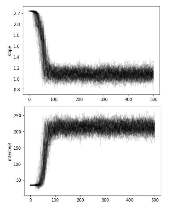
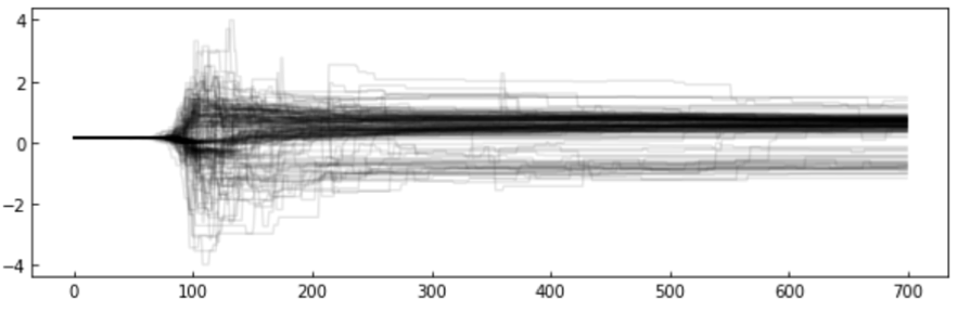
The chains: the algorithm creates a "chain" (a random walk) that "explores" the likelihood surface.
More efficient is to run many parallel chains - each exploring the surface, an "ensemble"
The path of the chains can be shown along each feature
choose a starting point in the parameter space: current = θ0 = (m0,b0)
WHILE convergence criterion is met:
calculate the current posterior pcurr = P(D|θ0,f)
//proposal
choose a new set of parameters new = θnew = (mnew,bnew)
calculate the proposed posterior pnew = P(D|θnew,f)
IF pnew/pcurr > 1:
current = new
ELSE:
//probabilistic step: accept with probability pnew/pcurr
draw a random number r ૯U[0,1]
IF r > pnew/pcurr >:
current = new
ELSE:
pass // do nothing
step
feature value
Examples of how to choose the next point
affine invariant : EMCEE package
choose a starting point in the parameter space: current = θ0 = (m0,b0)
WHILE convergence criterion is met:
calculate the current posterior pcurr = P(D|θ0,f)
//proposal
choose a new set of parameters new = θnew = (mnew,bnew)
calculate the proposed posterior pnew = P(D|θnew,f)
IF pnew/pcurr > 1:
current = new
ELSE:
//probabilistic step: accept with probability pnew/pcurr
draw a random number r ૯U[0,1]
IF r > pnew/pcurr >:
current = new
ELSE:
pass // do nothing
step
feature value
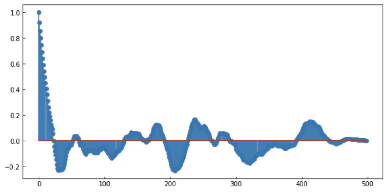
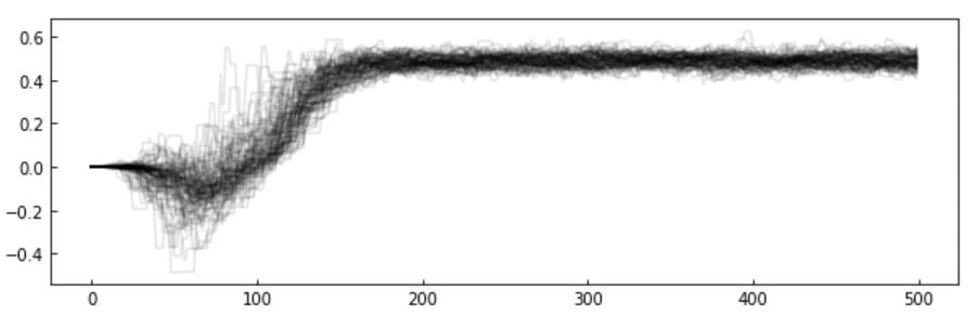
MCMC convergence
MCMC convergence
MCMC convergence
MCMC convergence
MCMC convergence
Point of change
3
detecting a change in the generative process:
the process is piecewise stationary
Key Concept
detecting a change in the generative process:
the process is piecewise stationary
examples:
Urban lights turn on-off transitions
to feed into energy demand models
and study urban life dynamics
detecting a change in the generative process:
the process is piecewise stationary
examples:
Urban lights turn on-off transitions
to feed into energy demand models
and study urban life dynamics
detecting a change in the generative process:
the process is piecewise stationary
examples:
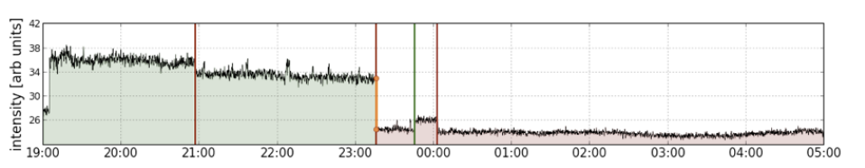
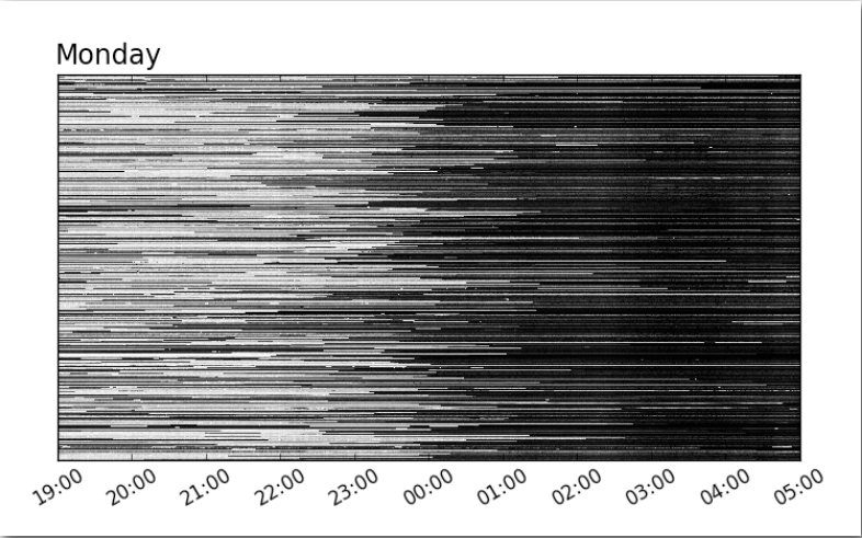
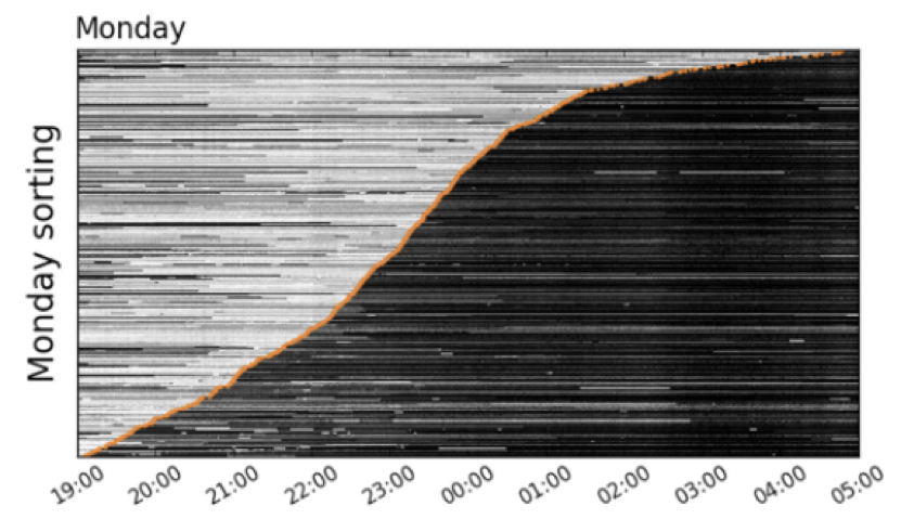
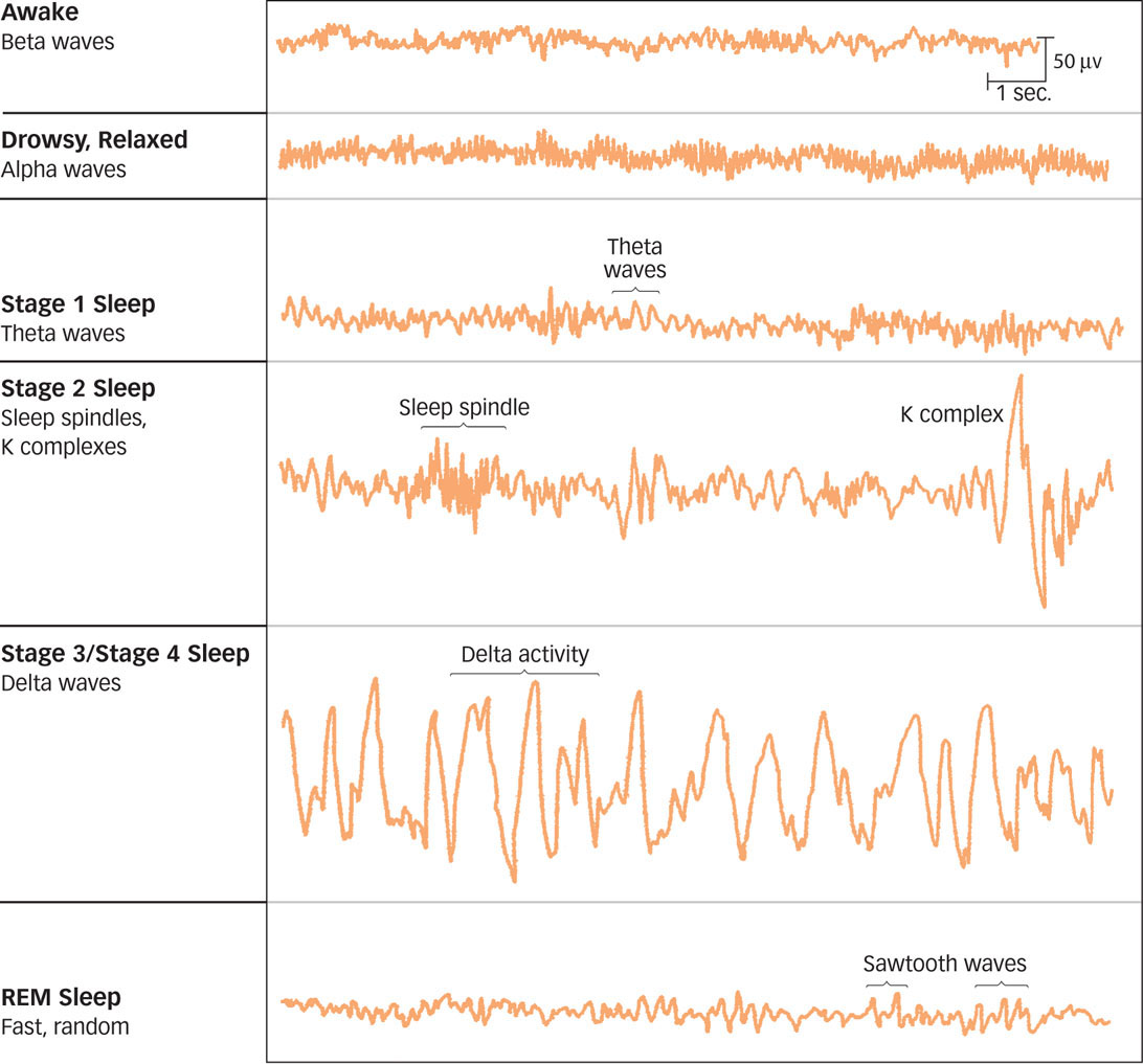
Brain wave transitions as different phases of sleep alternate
https://www.ncbi.nlm.nih.gov/pmc/articles/PMC5464762/#R52
Speech recognition represents the process of converting spoken speech utterances to words or text. Change point detection methods are applied here for audio segmentation and recognizing boundaries between silence, sentences, words, and noise [13][14].
Chowdhury MFR, Selouani SA, O’Shaughnessy D. Bayesian on-line spectral change point detection: a soft computing approach for on-line ASR. Int J Speech Technol. 2011 Oct;15(1):5–23. [Google Scholar]
Rybach D, Gollan C, Schluter R, Ney H. Audio segmentation for speech recognition using segment features. IEEE International Conference on Acoustics, Speech and Signal Processing. 2009:4197–4200. [Google Scholar]
detecting a change in the generative process:
the process is piecewise stationary
change in mean -> e.g. physics state transition
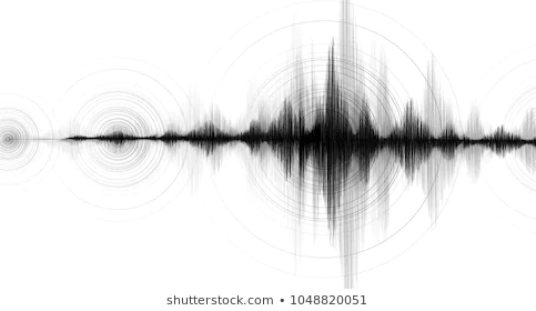
change in variance -> e.g. earthquake
detecting a change in the generative process:
the process is piecewise stationary
change in mean -> e.g. physics state transition
change in variance -> e.g. earthquake
online = in real time
when performed online POC analysis is equivalent to anomaly detection
offline = considering the whole time series
when performed offline POC analysis is equivalent to segmentation
DEFINITION:
Point of change:
Bayesian approach
3.1
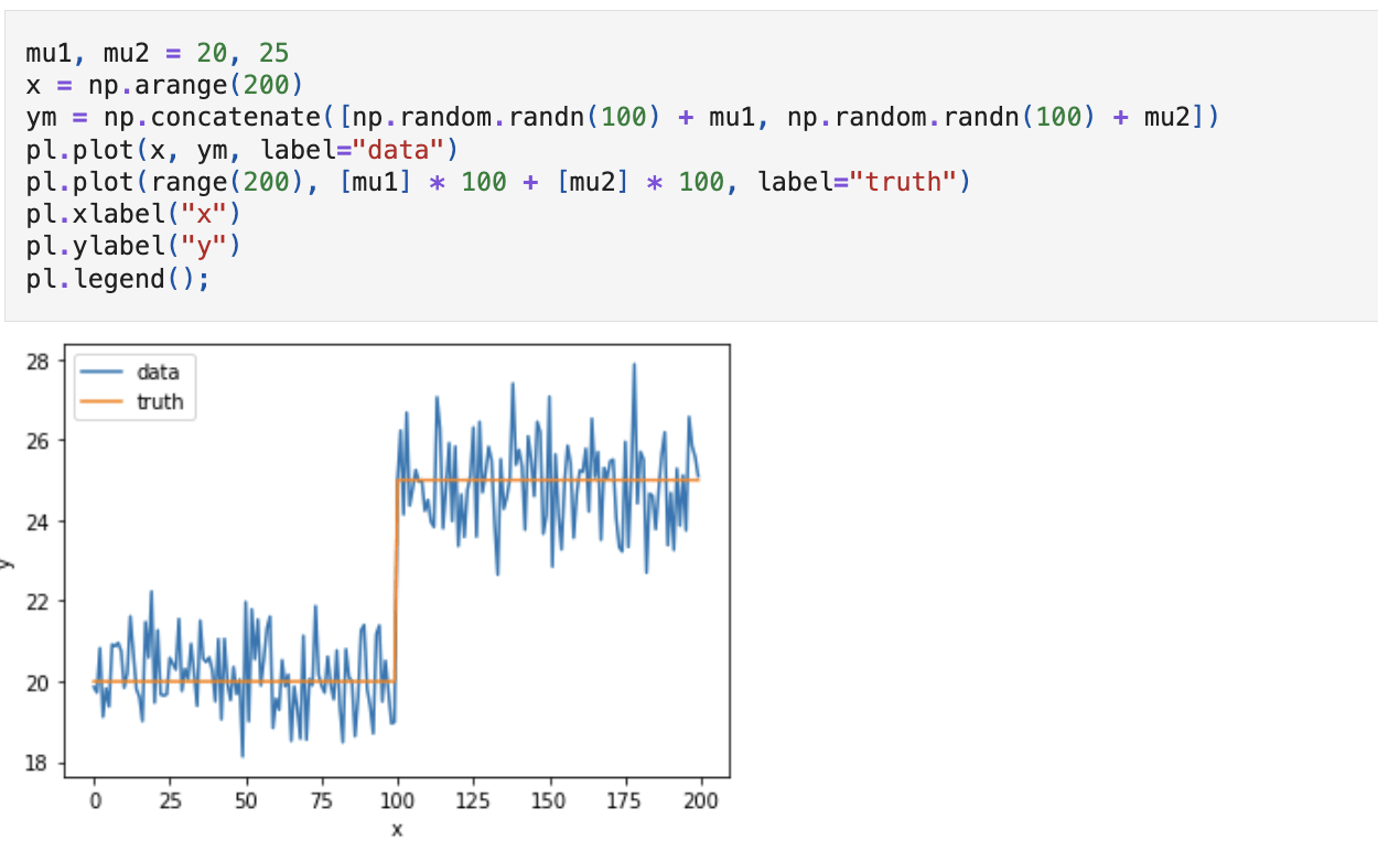
Suppose you know there is only one point of change, and that the change is only in the mean:
simplest approach
Frequentist approach
Bayesian approach
there is an unknown partition poc such that the distributions are equal within blocks
(assume iid, ~N... all nice things)
A Survey of Methods for Time Series Change Point Detection
Bayesian approach
A Survey of Methods for Time Series Change Point Detection
Bayesian approach
Really we want P(poc|D)
A Survey of Methods for Time Series Change Point Detection
Bayesian approach
Really we want P(poc|D)
Priors:
A Survey of Methods for Time Series Change Point Detection
Bayesian approach
Point of change:
n-points generalizatoin
3.2
the problem reduces to:
choosing the best possible segmentation T
such that a target function V (T , y) is minimized
(Ignores Bayesian approaches)
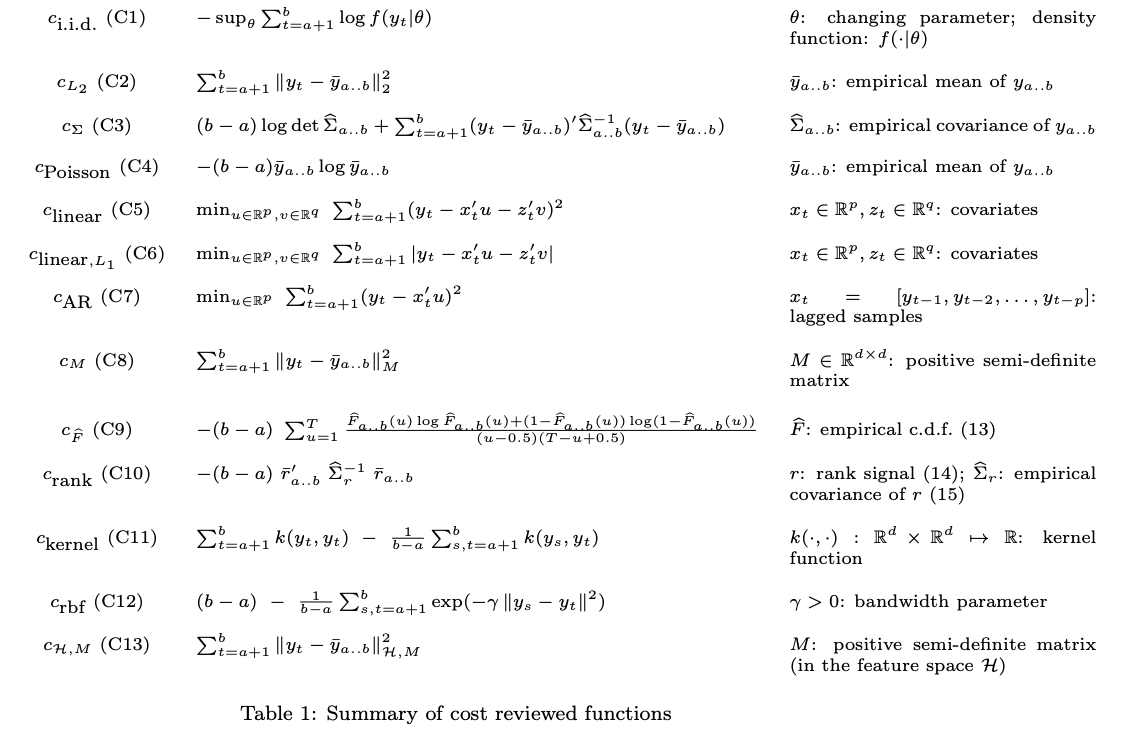
Selective review of offline change point detection methods
Charles Truonga, Laurent Oudre, Nicolas Vayatis
Formally, change point detection is cast as a model selection problem, which consists in choosing the best possible segmentation T according to a quantitative criterion V (T , y) that must be minimized. The choice of the criterion function V (·) depends on preliminary knowledge on the task at hand.
(Ignores Bayesian approaches)
Selective review of offline change point detection methods
Charles Truonga, Laurent Oudre, Nicolas Vayatis
(Ignores Bayesian approaches)
(Ignores Bayesian approaches)
Selective review of offline change point detection methods
Charles Truonga, Laurent Oudre, Nicolas Vayatis
(Ignores Bayesian approaches)
(Ignores Bayesian approaches)
Selective review of offline change point detection methods
Charles Truonga, Laurent Oudre, Nicolas Vayatis
1) toy model manual solution
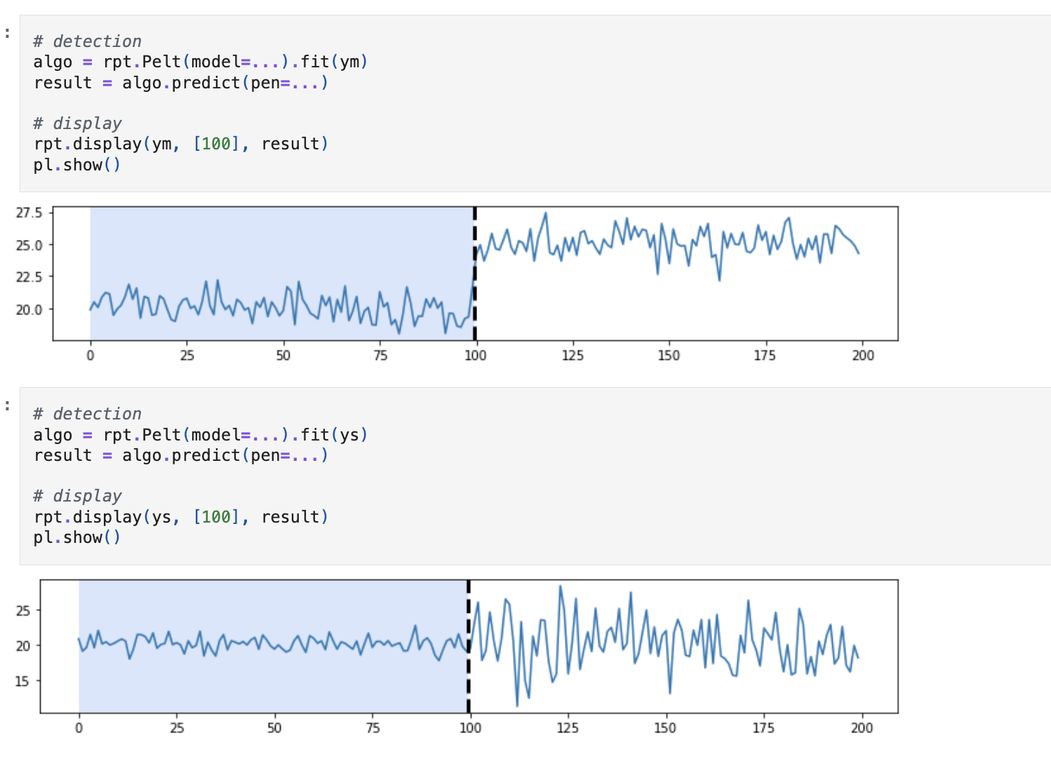
2) toy model using a module
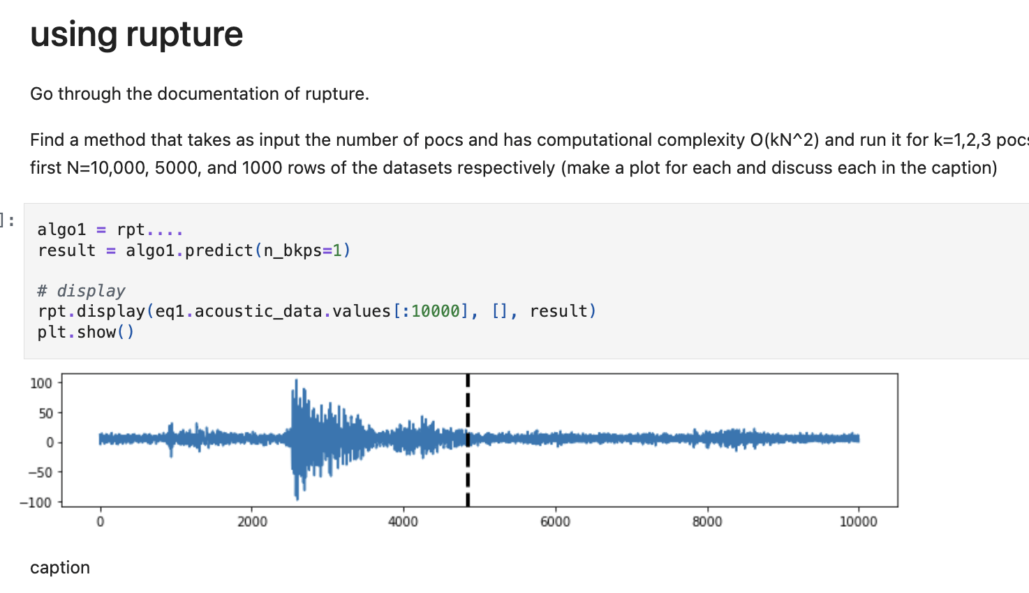
2) real data using a module
LR = _____________________________
True Negative
False Negative
| H0 is True | H0 is False | |
|---|---|---|
| H0 is falsified | Type I Error False Positive |
True Positive |
|
H0 is not falsified |
True Negative | Type II Error False Negative |
| H0 is True | H0 is False | |
|---|---|---|
| H0 is falsified | Type I Error False Positive |
True Positive |
|
H0 is not falsified |
True Negative | Type II Error False Negative |
Find a POC where there is none
miss a POC
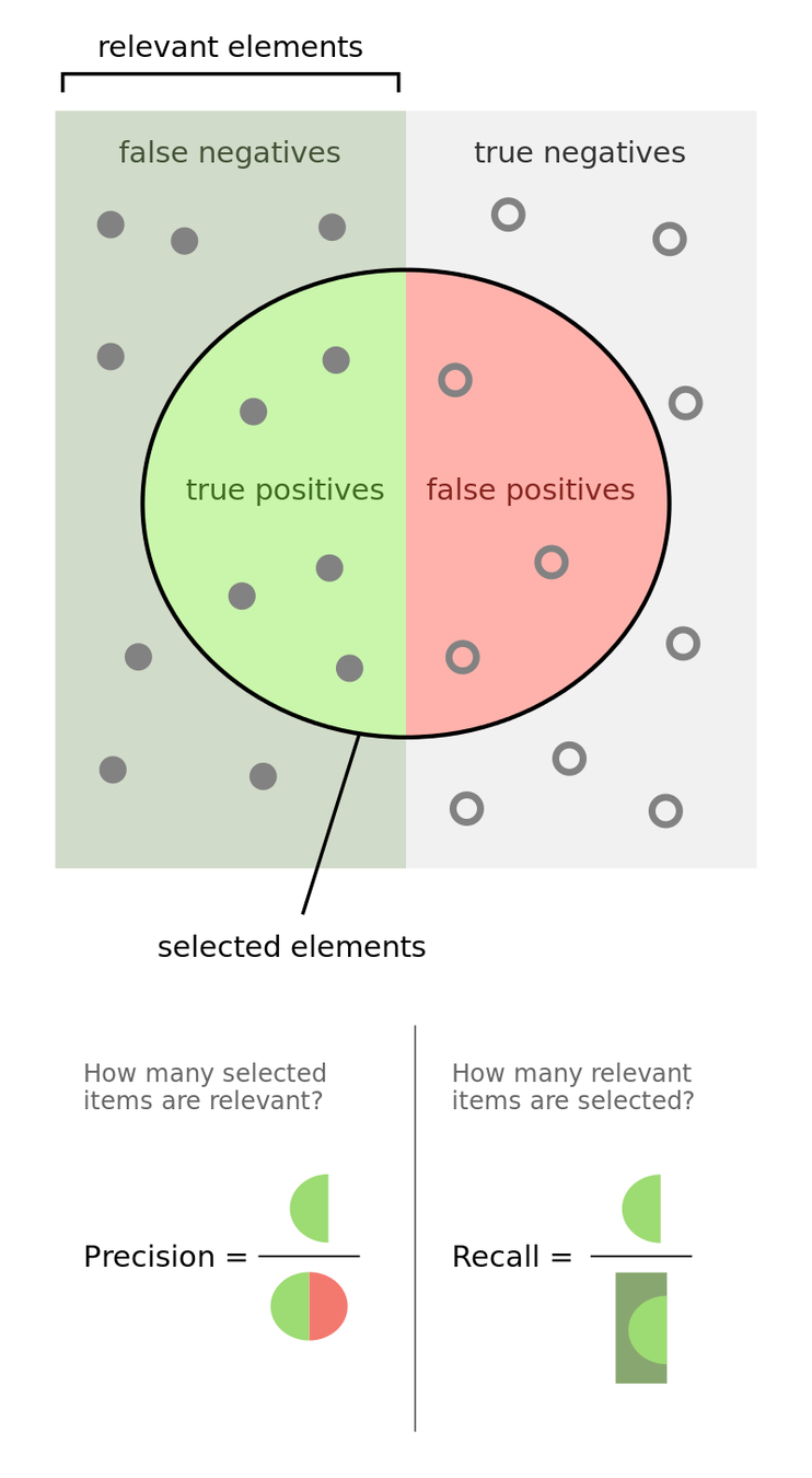
Precision
Recall
Accuracy
TP=True Positive
FP=False Positive
TN=True Negative
FN=False Positive
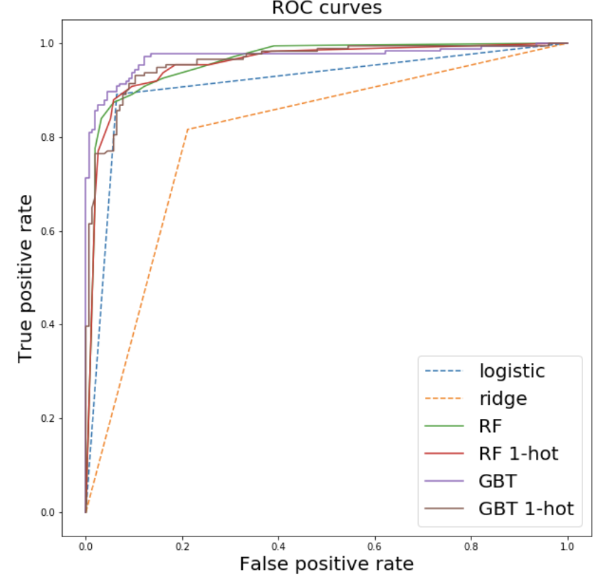
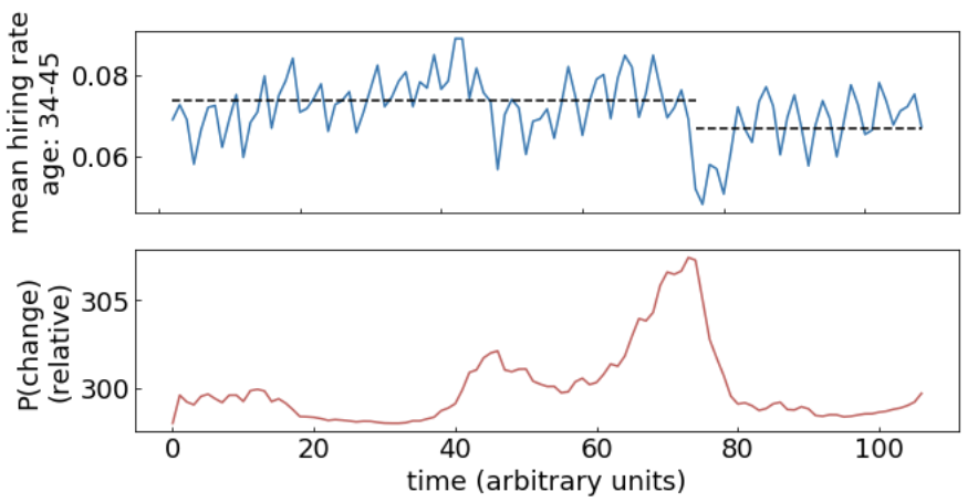
In a probabilistic context, as you change the probability threshold for selection of POC you will get a different FP TP ratio.
In a probabilistic context, as you change the probability threshold for selection of POC you will get a different FP TP ratio.
##single point change detector
# as in https://www.slideshare.net/FrankKelly3/changepoint-detection-with-bayesian-inference
# with modifications for efficiency

def changeFinder(data):

    n = len(data)
    datamean = data.mean()
    datasqmean = (data**2).mean()
    fac = datasqmean - datamean**2

    datacsum = data.cumsum()
    datasum = datacsum[-1]

    ppoc = np.zeros(n) #container for point of change relative prob

    #online (iterative) search for point of change
    for m in range(n-1):
        pos = m + 1
        relativePosition = (pos) * (n - pos)

        Q = datacsum[m] - (datasum - datacsum[m]) #cumsum up to m - cumsum after

        U = -(datamean * (n - 2 * pos) + Q)**2 / (4.0 * relativePosition) + fac

        ppoc[m+1] = (-(n * 0.5 - 1) * np.log(n * U * 0.5) -
                 0.5 * np.log(relativePosition))

    ppoc[0] = min(ppoc[1:])
    changePoint = np.argmax(ppoc)

    return {'pChange': ppoc,
            'pointOfChange': changePoint + 1,
            'meanBefore': (data[:changePoint+1]).mean(),
            'meanAfter': (data[(changePoint+1):]).mean()}
high FP rate
high TP rate
In a probabilistic context, as you change the probability threshold for selection of POC you will get a different FP TP ratio.
##single point change detector
# as in https://www.slideshare.net/FrankKelly3/changepoint-detection-with-bayesian-inference
# with modifications for efficiency

def changeFinder(data):

    n = len(data)
    datamean = data.mean()
    datasqmean = (data**2).mean()
    fac = datasqmean - datamean**2

    datacsum = data.cumsum()
    datasum = datacsum[-1]

    ppoc = np.zeros(n) #container for point of change relative prob

    #online (iterative) search for point of change
    for m in range(n-1):
        pos = m + 1
        relativePosition = (pos) * (n - pos)

        Q = datacsum[m] - (datasum - datacsum[m]) #cumsum up to m - cumsum after

        U = -(datamean * (n - 2 * pos) + Q)**2 / (4.0 * relativePosition) + fac

        ppoc[m+1] = (-(n * 0.5 - 1) * np.log(n * U * 0.5) -
                 0.5 * np.log(relativePosition))

    ppoc[0] = min(ppoc[1:])
    changePoint = np.argmax(ppoc)

    return {'pChange': ppoc,
            'pointOfChange': changePoint + 1,
            'meanBefore': (data[:changePoint+1]).mean(),
            'meanAfter': (data[(changePoint+1):]).mean()}
low FP rate
low TP rate
In a probabilistic context, as you change the probability threshold for selection of POC you will get a different FP TP ratio.
##single point change detector
# as in https://www.slideshare.net/FrankKelly3/changepoint-detection-with-bayesian-inference
# with modifications for efficiency

def changeFinder(data):

    n = len(data)
    datamean = data.mean()
    datasqmean = (data**2).mean()
    fac = datasqmean - datamean**2

    datacsum = data.cumsum()
    datasum = datacsum[-1]

    ppoc = np.zeros(n) #container for point of change relative prob

    #online (iterative) search for point of change
    for m in range(n-1):
        pos = m + 1
        relativePosition = (pos) * (n - pos)

        Q = datacsum[m] - (datasum - datacsum[m]) #cumsum up to m - cumsum after

        U = -(datamean * (n - 2 * pos) + Q)**2 / (4.0 * relativePosition) + fac

        ppoc[m+1] = (-(n * 0.5 - 1) * np.log(n * U * 0.5) -
                 0.5 * np.log(relativePosition))

    ppoc[0] = min(ppoc[1:])
    changePoint = np.argmax(ppoc)

    return {'pChange': ppoc,
            'pointOfChange': changePoint + 1,
            'meanBefore': (data[:changePoint+1]).mean(),
            'meanAfter': (data[(changePoint+1):]).mean()}
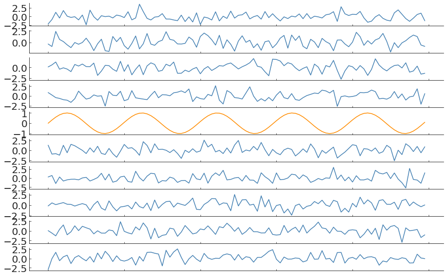
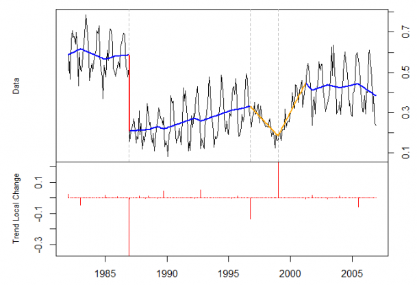
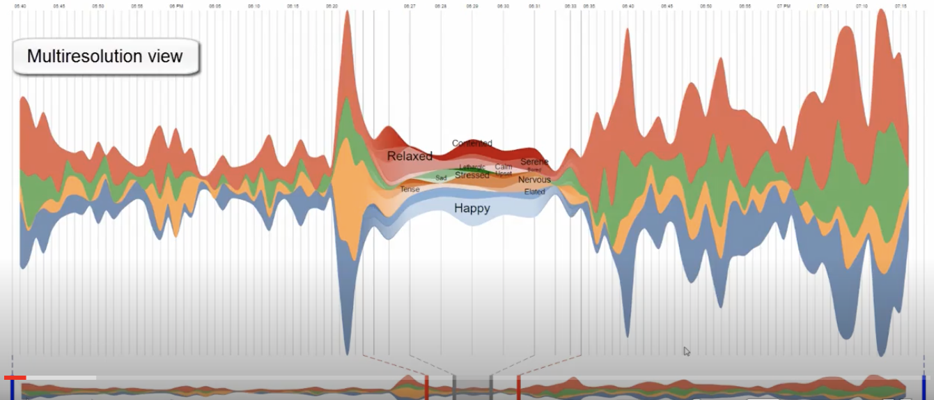
This plot style is a "stream graph".
They are good for multivariate data as they enable the comparison of several (but not too many) time series.
Overall changes in volume (and therefore the variance) is going to be more obvious than trends.
This plot style is a "stream graph".
This particular image is a screenshot from an interactive tool
http://advanse.lirmm.fr/hierarchical/visualize.php
When you design an interactive tool you want to keep two principles in mind
1. The tool should show context/overview first, details should be available on demand (in this tool you can select a portion of the time series and expand it)
2. Access to details should be immediate: people are really patient... for 3 seconds. Then they loose interest and attention
The Unofficial Google Data Science Blog
http://www.unofficialgoogledatascience.com/2017/07/fitting-bayesian-structural-time-series.html
Matlab Kalman Filter tutorial videos (super clear!) https://www.youtube.com/watch?v=mwn8xhgNpFY
A Survey of Methods for Time Series Change Point Detection
Samaneh Aminikhanghahi and Diane J. Cook
Selective review of offline change point detection methods
Charles Truonga, Laurent Oudre, Nicolas Vayatis
Selective review of offline change point detection methods
Charles Truonga, Laurent Oudre, Nicolas Vayatis
Choose any one method and one cost function described in this paper and read about it in detail. You should be prepared to
write the cost function, describe it, discuss the merit of the method and its applications (e.g. is it good for 1 poc or N poc? ) quizzes may contain questions about this
Point of change detection and validation in Earthquake detection
By federica bianco
Anomaly detection and Point of Change Detection


