


federica bianco PRO
astro | data science | data for good
Fall 2025 - UDel PHYS 661
dr. federica bianco
@fedhere
this slide deck:
supervised vs unsupervised learning
1
classification
prediction
feature selection
supervised learning
understanding structure
organizing/compressing data
anomaly detection dimensionality reduction
unsupervised learning
classification
prediction
feature selection
supervised learning
understanding structure
organizing/compressing data
anomaly detection dimensionality reduction
unsupervised learning
clustering
PCA
Apriori
k-Nearest Neighbors
Regression
Support Vector Machines
Classification/Regression Trees
Neural networks
observed features:
(x, y)
GOAL: partitioning data in maximally homogeneous,
maximally distinguished subsets.
x
y
all features are observed for all objects in the sample
(x, y)
how should I group the observations in this feature space?
e.g.: how many groups should I make?
x
y
all features are observed for all objects in the sample
(x, y)
how should I group the observations in this feature space?
e.g.: how small can clusters get?
x
y
unsupervised learning methods
(clustering)
find partitions of the space to discover structure
used to:
understand structure of feature space
x
y
observed features:
(x, y)
models typically return a partition of the space
goal is to partition the space so that the unobserved variables are
separated in groups
consistently with
an observed subset
target features:
(color)
t
y
observed features:
(x, y)
ax+b
if y <= a*t + b :
	return blue
else:
	return orange
target features:
(color)
t
y
observed features:
(x, y)
if t**2 + y**2 <= (t-a)**2 + (y-b)**2 :
	return blue
else:
	return orange
target features:
(color)
supervised learning methods
(nearly all other methods you heard of)
learns by example
used to:
classify, predict (regression)
t
y
observed features:
(x, y)
Tree Methods
split spaces along each axis separately
A subset of variables has class labels. Guess the label for the other variables
split along x
if t <= a :
	return blue
else:
	return orange
target features:
(color)
t
y
observed features:
(x, y)
Tree Methods
split spaces along each axis separately
A subset of variables has class labels. Guess the label for the other variables
split along x
if t <= a :
	if y <= b:
      		return blue
return orange
then
along y
target features:
(color)
t
y
observed features:
(x, y)
A subset of variables has class labels. Guess the label for the other variables
split along x
if x <= a :
	if y <= b:
      		return blue
return orange
then
along y
target features:
(color)
this makes it ideal when you have hybrid feature types (e.g. numerical vs categorical)
Tree Methods
split spaces along each axis separately
Tree Methods
example of supervised learning method
partitions feature space along each feature separately
The good
The bad
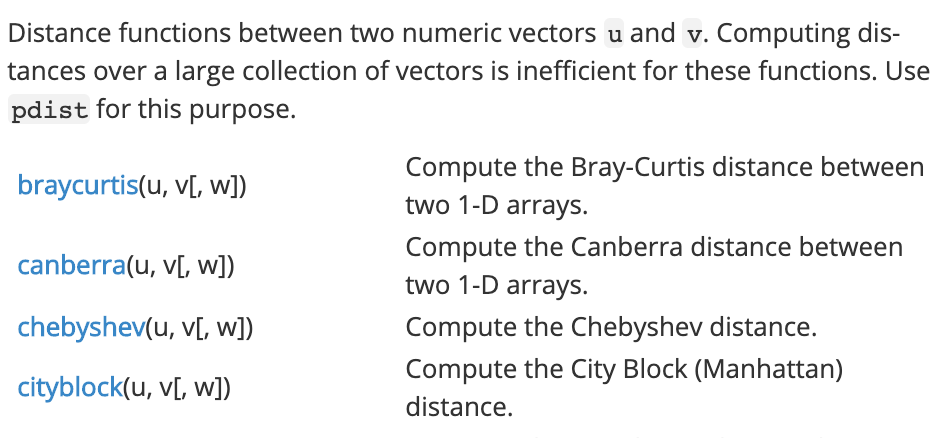
distances
2
Minkowski family of distances
Minkowski family of distances
L1 is the Minkowski distance with p=1
L2 is the Minkowski distance with p=2
Minkowski family of distances
N features (dimensions)
Minkowski family of distances
N features (dimensions)
properties:
Minkowski family of distances
Manhattan: p=1
features: x, y
Minkowski family of distances
Manhattan: p=1
features: x, y
Minkowski family of distances
Euclidean: p=2
features: x, y
Minkowski family of distances
L1 is the Minkowski distance with p=1
L2 is the Minkowski distance with p=2
Residuals
3
3
2
2
2
Minkowski family of distances
L1 is the Minkowski distance with p=1
L2 is the Minkowski distance with p=2
Residuals
2
2
3
2
2
3
L1 = 7
Minkowski family of distances
L1 is the Minkowski distance with p=1
L2 is the Minkowski distance with p=2
Residuals
2
2
3
L1 = 7
L2 = 17
Minkowski family of distances
Great Circle distance
features
latitude and longitude
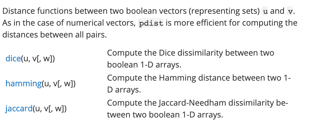
Uses presence/absence of features in data
: number of features in neither
: number of features in both
: number of features in i but not j
: number of features in j but not i
| 1 | 0 | sum | |
|---|---|---|---|
| 1 | M11 | M10 | M11+M10 |
| 0 | M01 | M00 | M01+M00 |
| sum | M11+M01 | M10+M00 | M11+M00+M01+ M10 |
observation i
observation j
}
}
Simple Matching Distance
Uses presence/absence of features in data
: number of features in neither
: number of features in both
: number of features in i but not j
: number of features in j but not i
Simple Matching Coefficient
or Rand similarity
| 1 | 0 | sum | |
|---|---|---|---|
| 1 | M11 | M10 | M11+M10 |
| 0 | M01 | M00 | M01+M00 |
| sum | M11+M01 | M10+M00 | M11+M00+M01+ M10 |
observation i
observation j
}
}
Jaccard similarity
Jaccard distance
| 1 | 0 | sum | |
|---|---|---|---|
| 1 | M11 | M10 | M11+M10 |
| 0 | M01 | M00 | M01+M00 |
| sum | M11+M01 | M10+M00 | M11+M00+M01+ M10 |
observation i
observation j
}
}
Jaccard similarity
Jaccard distance
| 1 | 0 | sum | |
|---|---|---|---|
| 1 | M11 | M10 | M11+M10 |
| 0 | M01 | M00 | M01+M00 |
| sum | M11+M01 | M10+M00 | M11+M00+M01+ M10 |
observation i
observation j
}
}
distance in time series
2.1
distance in time series
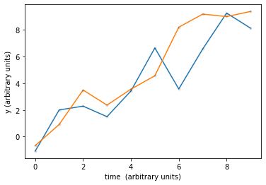
simple time series distance:
Euclidean point by point
distance in time series
simple time series distance:
Euclidean point by point
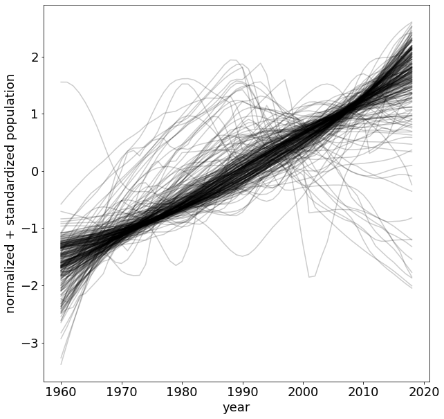
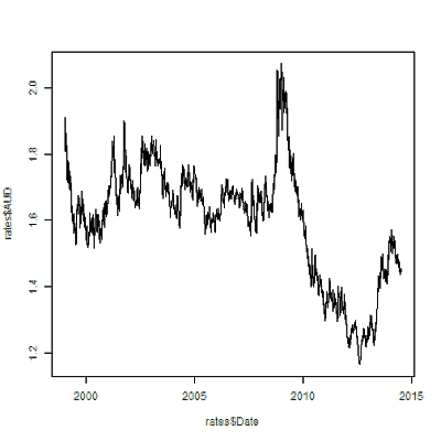
distance in time series
https://data.worldbank.org/indicator/SP.POP.TOTL
distance in time series
time series are vectors
example of distance metric that works on vectors:
correlation coefficient r
distance in time series
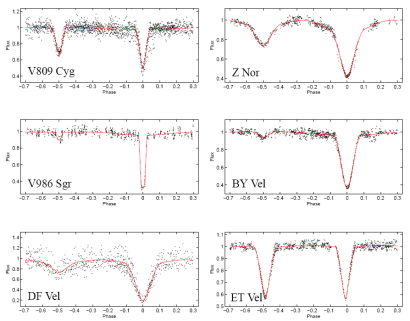
how similar is similar? these time series are of the same phenomenon: eclipsing binaries. But they look different enough that it would be hard to write a classifier that recognizes this
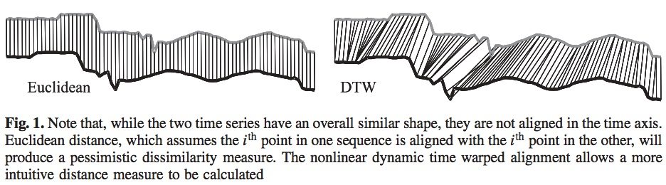
distance in time series
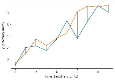
what if the time series is shifted? : these are identical time series shifted along the x axis. The correlation coefficient would be low tho!
distance in time series
what if the time series is shifted? : these are identical time series shifted along the x axis. The correlation coefficient would be low tho!
what if the time series is stretched? : these are identical time series but the top one is stretched. Similarly the
distance in time series
One possible approach: DTW algorithm
Dynamic Time Warping (future class maybe?)
distance in time series
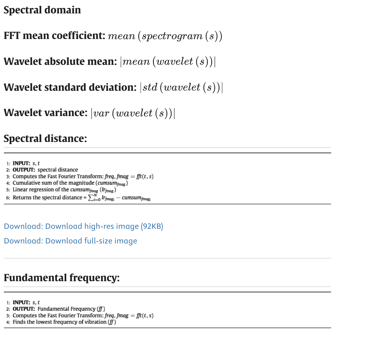
Another approach: learn features from data and measure distance between those
st deviation, min-max distance,
peaks in frequency space....
CART
classification and regression trees
3
Application:
a robot to predict surviving the Titanic
714 passengers Ns=424 Nd=290
features:
target variable:
-> survival (y/n)
gender (binary)
M
Ns=93 Nd=360
F
Ns=197 Nd=64
Application:
a robot to predict surviving the Titanic
714 passengers Ns=424 Nd=290
features:
target variable:
-> survival (y/n)
gender (binary)
M
Ns=93 Nd=360
F
Ns=197 Nd=64
optimize over purity:
Application:
a robot to predict surviving the Titanic
714 passengers Ns=424 Nd=290
features:
target variable:
-> survival (y/n)
gender (binary)
M
Ns=93 Nd=360
F
Ns=197 Nd=64
optimize over purity:
Application:
a robot to predict surviving the Titanic
714 passengers Ns=424 Nd=290
features:
target variable:
-> survival (y/n)
1st
Ns=120 Nd=80
2nd +3rd
Ns=234 Nd=298
class (ordinal)
Application:
a robot to predict surviving the Titanic
714 passengers Ns=424 Nd=290
features:
target variable:
-> survival (y/n)
age (continuous)
>6.5
Ns=250 Nd=107
<=6.5
Ns=139 Nd=217
Application:
a robot to predict surviving the Titanic
714 passengers Ns=424 Nd=290
target variable:
-> survival (y/n)
gender (binary)
M
Ns=93 Nd=360
F
Ns=197 Nd=64
features:
Application:
a robot to predict surviving the Titanic
714 passengers Ns=424 Nd=290
target variable:
-> survival (y/n)
gender (binary)
M
Ns=93 Nd=360
F
Ns=197 Nd=64
features:
Application:
a robot to predict surviving the Titanic
714 passengers Ns=424 Nd=290
target variable:
-> survival (y/n)
gender
M
Ns=93 Nd=360
F
Ns=197 Nd=64
age
>6.5
Ns=250 Nd=107
<=6.5
Ns=139 Nd=217
class
1st + 2nd
Ns=120 Nd=80
3rd
Ns=234 Nd=298
features:
Application:
a robot to predict surviving the Titanic
714 passengers Ns=424 Nd=290
target variable:
-> survival (y/n)
gender
M
Ns=93 Nd=360
F
Ns=197 Nd=64
age
>6.5
Ns=250 Nd=107
p=82%
<=6.5
Ns=139 Nd=217
p=67%
class
age
>2.5
Ns=1 Nd=1
p=50%
<=2,5
Ns=8 Nd=139
p=95%
age
>38.5
Ns=44 Nd=46
<=38.5
Ns=11 Nd=1
1st + 2nd
Ns=120 Nd=80
3rd
Ns=234 Nd=298
features:
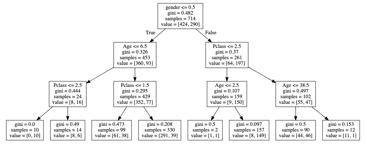
Application:
a robot to predict surviving the Titanic
714 passengers Ns=424 Nd=290
features:
target variable:
-> survival (y/n)
gender
M
Ns=93 Nd=360
F
Ns=197 Nd=64
>6.5
Ns=250 Nd=107
p=82%
<=6.5
Ns=139 Nd=217
p=67%
1st + 2nd
Ns=120 Nd=80
3rd
Ns=234 Nd=298
1st
Ns=100 Nd=20
p=80%
2nd
Ns=40 Nd=40
p=50%
age
>38.5
Ns=44 Nd=46
<=38.5
Ns=11 Nd=1
class
age
class
A single tree
nodes
(make a decision)
root node
branches
(split off of a node)
leaves (last groups)
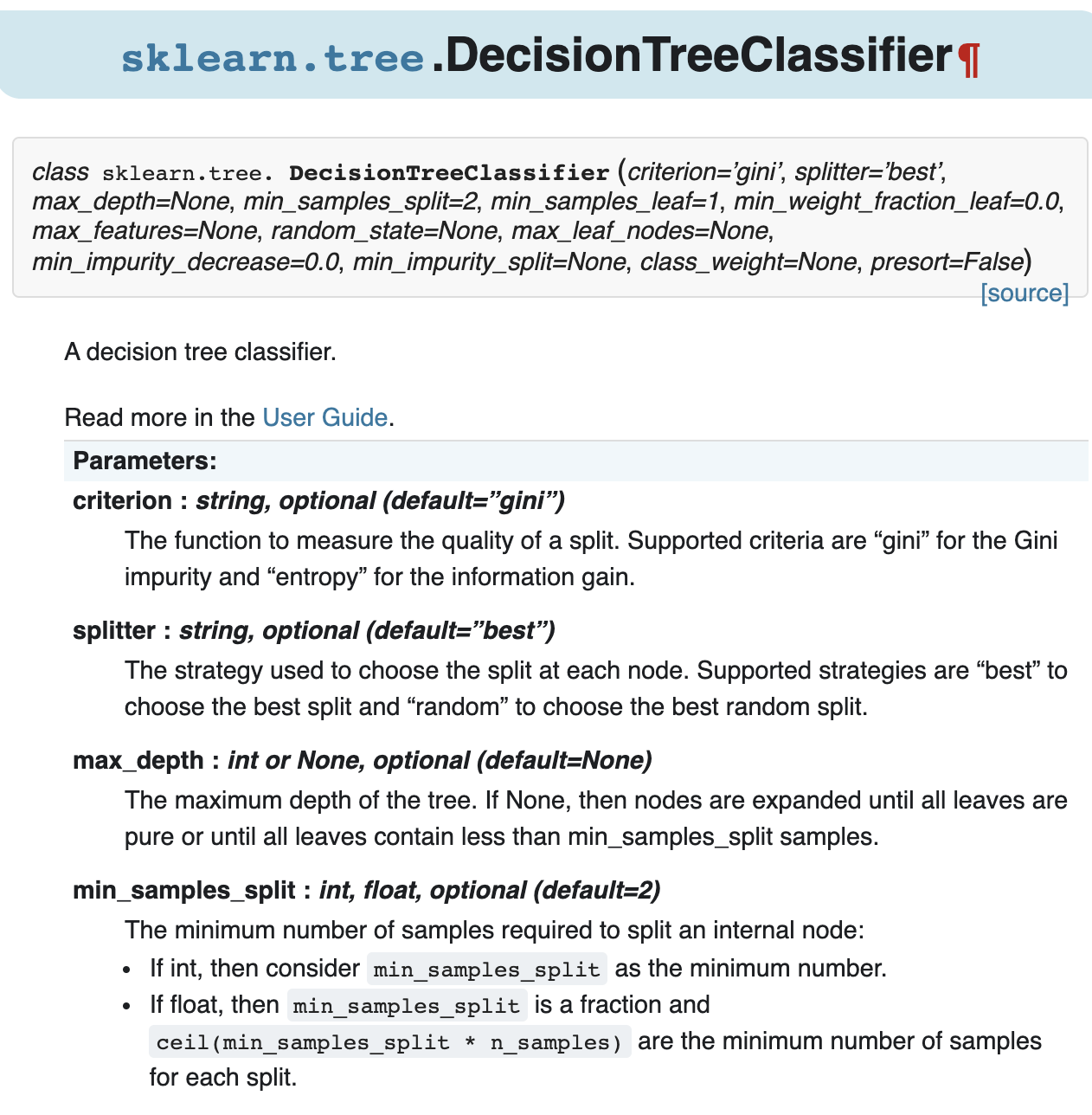
gini impurity
information gain (entropy)
A single tree: hyperparameters
depth
A single tree: hyperparameters
max depth = 2
A single tree: hyperparameters
max depth = 2
PREVENTS OVERGFITTING
A single tree: hyperparameters
alternative: tree pruning
A single tree: hyperparameters
CART: Classification and Regression Trees
variance:
different trees lead to different results
variance:
different trees lead to different results
why?
because calculating the criterion for every split and every mote is an untractable problem!
e.g. 2 coutinuous variables would be a problem of order
variance:
different trees lead to different results
solution
run many trees and take an "ensamble" decision!
Random Forests
Gradient Boosted Trees
a bunch of parallel trees
a series of trees
Gradient boosted trees:
trees run in series (one after the other)
each tree uses different weights for the features learning the weighs from the previous tree
the last tree has the prediction
Random forest:
trees run in parallel (independently of each other)
each tree uses a random subset of observations/features (boostrap - bagging)
class predicted by majority vote:
what class do most trees think a point belong to
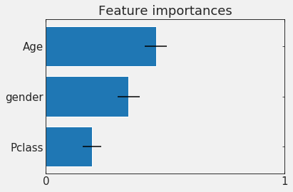
In principle CART methods are interpretable
you can measure the influence that each feature has on the decision : feature importance
In principle CART methods are interpretable
you can measure the influence that each feature has on the decision : feature importance
In practice the interpretation is complicated by covariance of features
Extraction of features
3
Consider a classification task:
if I want to use machine learning methods I need to choose:
use raw representation:
e.g. clustering:
1) take each time series and standardize it
(mean 0 standard 1).
2) for each time stamps compare them to the expected value (mean and stdev)
essentially each datapoint is treated as a feature
Consider a classification task:
if I want to use machine learning methods (e.g. clustering) I need to choose:
use raw representation
1) take each time series and standardize it (μ=0 ; σ=1).
2) for each time stamps compare them to the expected value (μ & σ)
problems:
(in small dataset you can optimize over warping and shifting but in large dataset this solution is computationally limited)
essentially each datapoint is treated as a feature
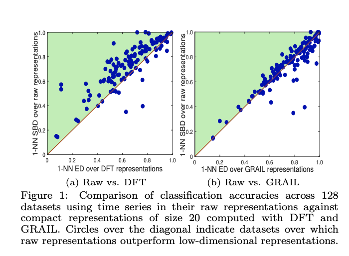
Consider a classification task:
if I want to use machine learning methods (e.g. clustering) I need to choose:
choose a low dimensional representation
essentially each datapoint is treated as a feature
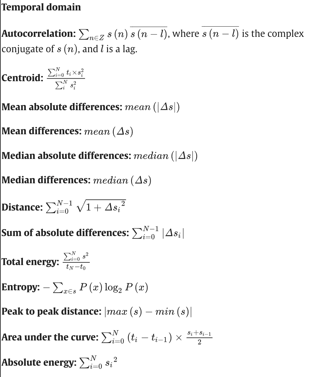
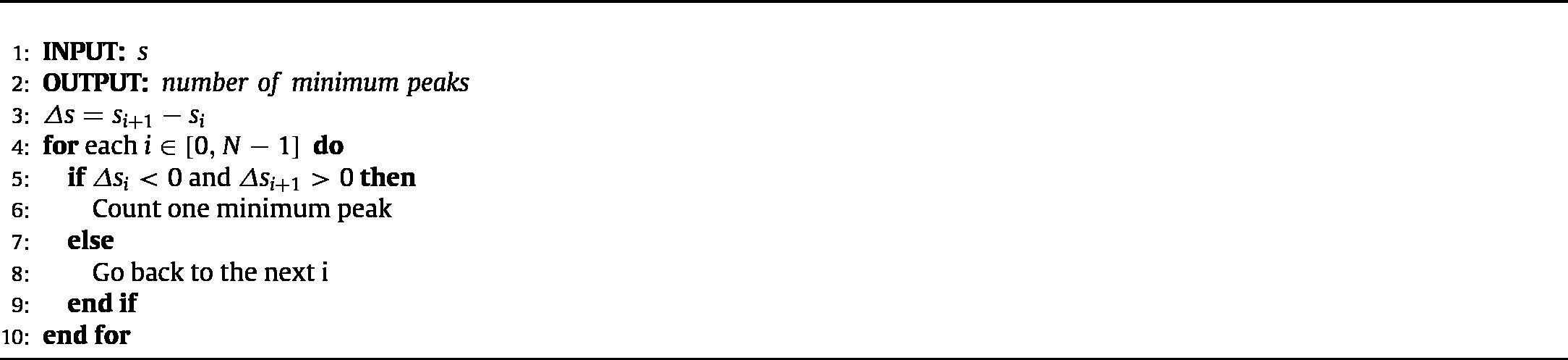
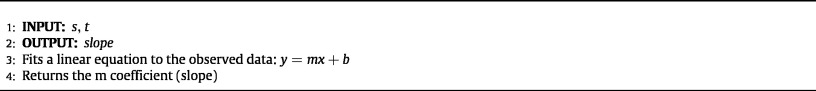
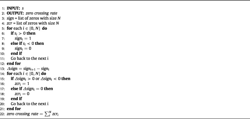
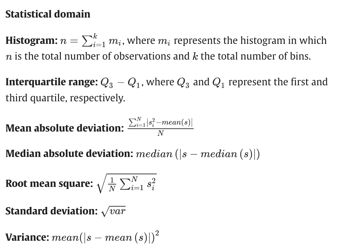
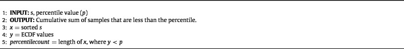
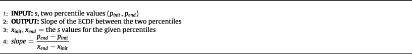
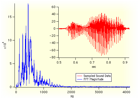
Extract features that describe the time series:
simple descriptive statistics (look at the distribution of points, regardless of the time evolution:
parametric features (based on fitting model to data):
Consider a classification task:
the learned representations should:
a comprehensive review of clustering methods
Data Clustering: A Review, Jain, Mutry, Flynn 1999
https://www.cs.rutgers.edu/~mlittman/courses/lightai03/jain99data.pdf
a blog post on how to generate and interpret a scipy dendrogram by Jörn Hees
https://joernhees.de/blog/2015/08/26/scipy-hierarchical-clustering-and-dendrogram-tutorial/
clustering
a model that uses clustering to generate features http://www.vldb.org/pvldb/vol12/p1762-paparrizos.pdf
a blog post on how to generate and interpret a scipy dendrogram by Jörn Hees
https://joernhees.de/blog/2015/08/26/scipy-hierarchical-clustering-and-dendrogram-tutorial/
Clustering : unsupervised learning where all features are observed for all datapoints. The goal is to partition the space into maximally homogeneous maximally distinguished groups
clustering is easy, but interpreting results is tricky
Distance : A definition of distance is required to group observations/ partition the space.
Common distances over continuous variables
Common distances over categorical variables:
Clustering : k-means - pros: its efficient and intuitive, cons: only works on euclidean distance, need to know the number of clusters
hierarchical: cons: less efficient, pros: provides the full length clustering tree
http://what-when-how.com/artificial-intelligence/decision-tree- applications-for-data-modelling-artificial-intelligence/
https://www.ncbi.nlm.nih.gov/pmc/articles/PMC4466856/
CART
Machine Learning includes models that learn parameters from data
ML models have parameters learned from the data and hyperparameters assigned by the user.
Unsupervised learning:
Supervised learning:
Tree methods:
Distributed and parallel time series feature extraction for industrial big data applications
Maximilian Christ a , Andreas W. Kempa-Liehrb,c, Michael Fein
https://arxiv.org/pdf/1610.07717.pdf
TL;DR:
Feature extractions from time series
Feature extractions from time series
Reading
Sections 1-2
Homework
Reproduce the class lab
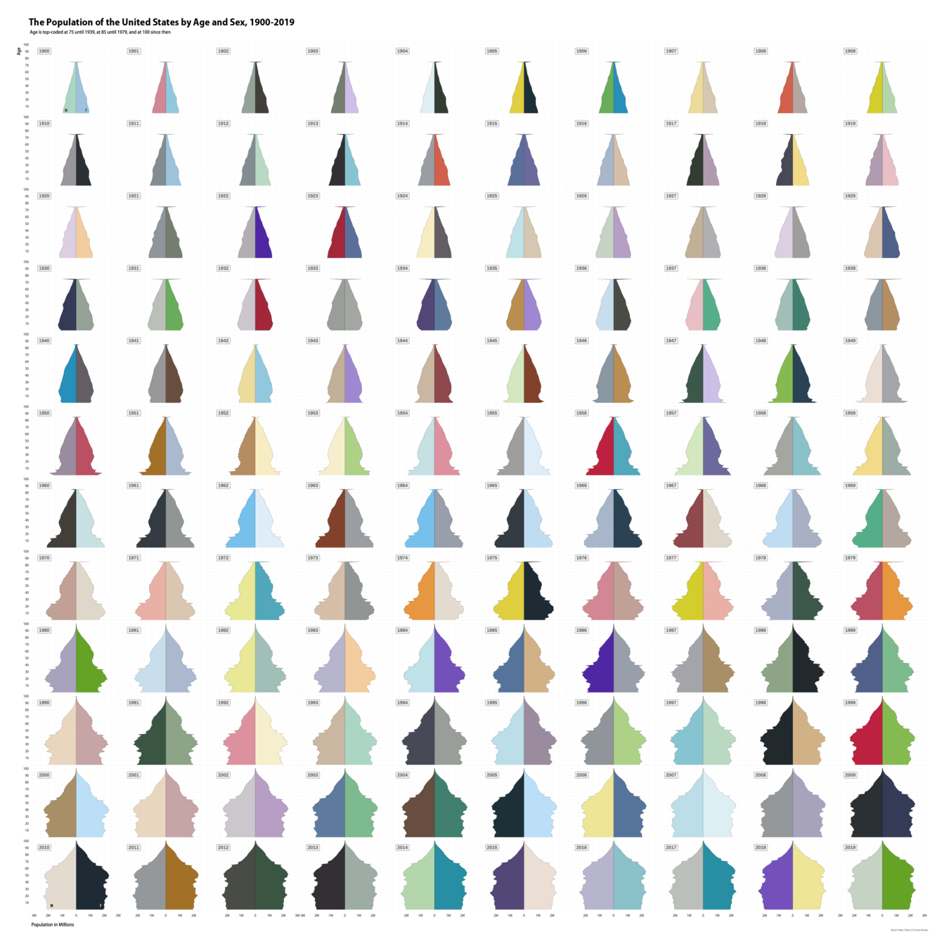
Visualization of the week
Kieran Healy https://kieranhealy.org/
By federica bianco
feature bases methods


