


federica bianco PRO
astro | data science | data for good
Fall 2025 - UDel PHYS 661
dr. federica bianco
@fedhere
this slide deck:
missing data
1
What to do if you have missing data?
- most models will fail
- statistics will be messed up
reminder: Stochastic process
A random variable indexed by time.
For any subset of points in time the dependent variable follows the a probability distribution
e.g.
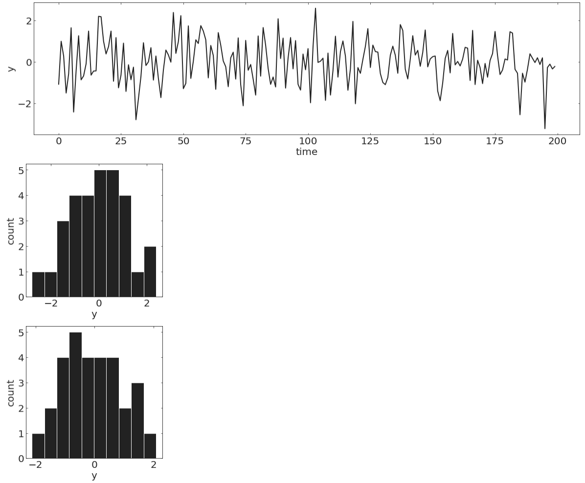
pl.figure(figsize=(20,5))
N = 200
np.random.seed(100)
y = np.random.randn(N)
t = np.linspace(0, N, N, endpoint=False)
pl.plot(t, y, lw=2)
pl.xlabel("time")
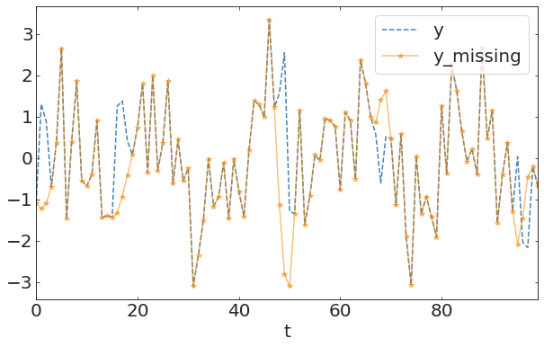
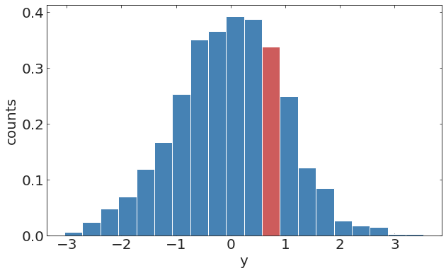
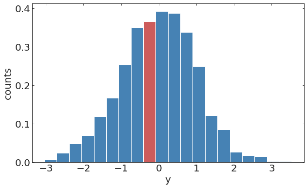
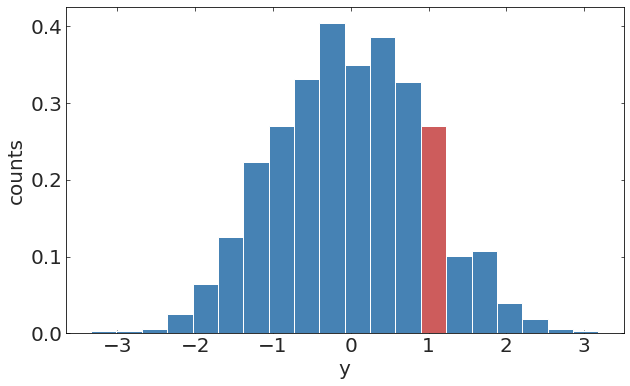
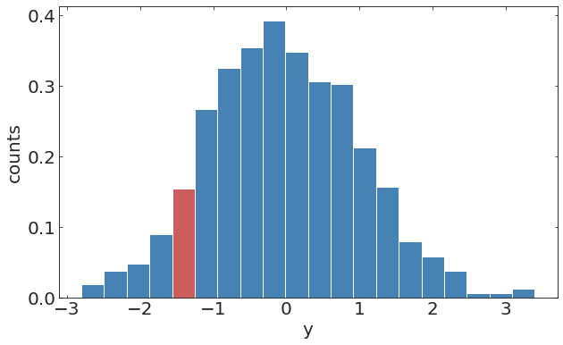
pl.ylabel("y");Discrete time stochastic process
pl.hist(y[20:70])pl.hist(y[100:150])randomely distributed missing observation
e.g. on off times of sensors
aggregate statistics should be preserved if the process is stockastic
missing data due to sensors' sensitivity
e.g. CCD cameras: need minimum light to generate signal
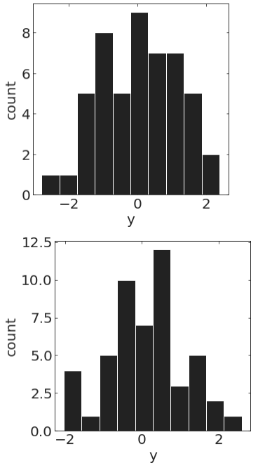
censored data (upper or lower limits)
aggregate statistics will be biased - specifically variance will always be suppresses
data aggregated above or below a threshold
e.g. medical records of people older than 90 are often aggregated as >90.
aggregate statistics will be biased - specifically variance will always be suppresses
censored data (upper or lower limits)
pandas imputation methods
- most models will fail
most models do not work with missing data
data imputation
2
Impute data with mean:
if your goal was to estimate the mean you may be ok. if your goal was to estimate the variance you have effectively suppressed it
Data imputation:
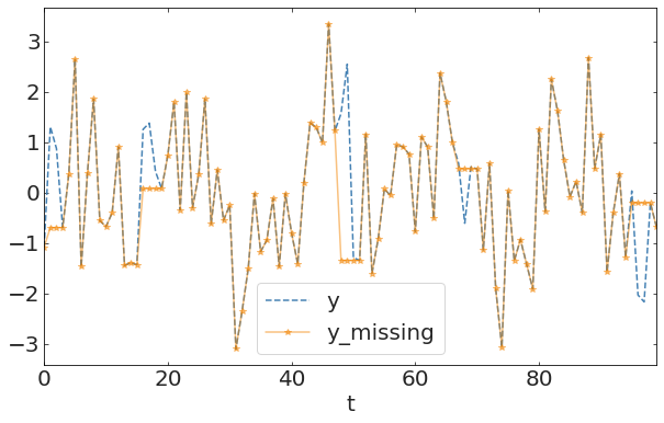
Fill in missing data and generating data at regular intervals of the exogenous variable (really important since most time-domain models require data to be evenly sampled)
Impute data with mean:
if your goal was to estimate the mean you may be ok. if your goal was to estimate the variance you have effectively suppressed it. In time domain it may cause significant jumps.
A local mean would be better tho.
Backward and forward filling:
particularly dangerous with time series analysis. You are implying stability in the system at scales where there is no statbility!
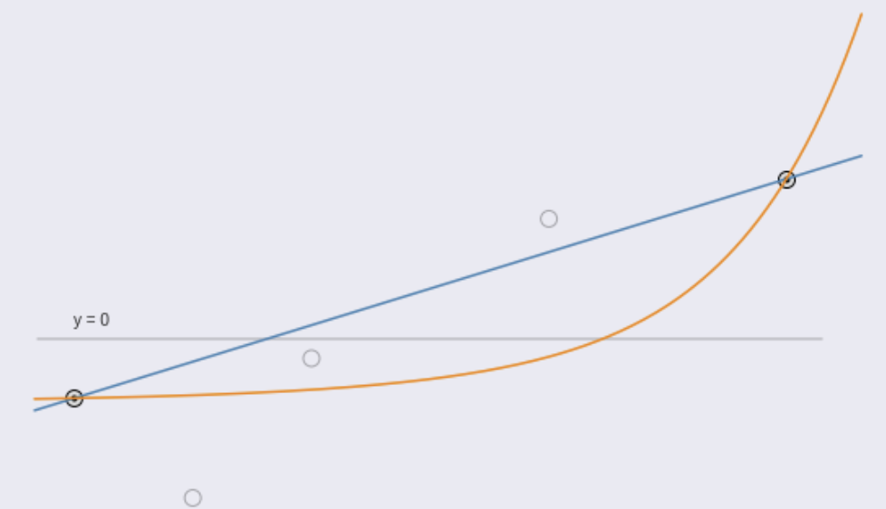
Linear, Cubic, Quadratic interpolation. Its model dependent. Unless you have a reason for the model you are constraining the data and will not likely get a food fit. Incerased flexibility in the model allows a better fit but exposes to overfitting risk
linear interpolation
quadratic interpolation
Parameteric (simlpe) approach - define a functional form (e.g. linear).
Data imputation requires definition of a function:
linear fit
10th degree polynomial fit
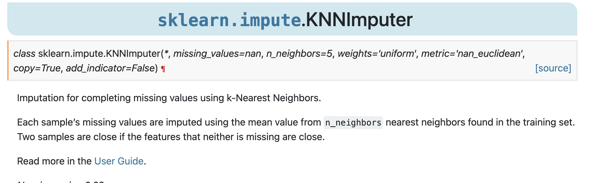
Can use Nearest Neighbor algorithm to impute. Thinking about time series in particular, this could be done along the time or along the feature axis
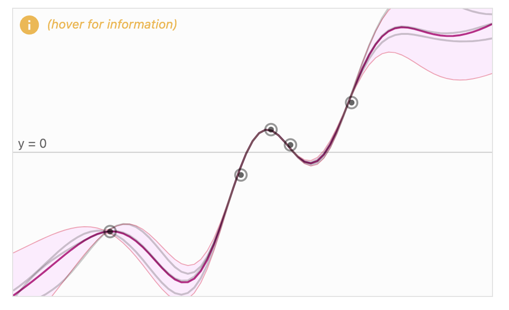
Gaussian Processes
3
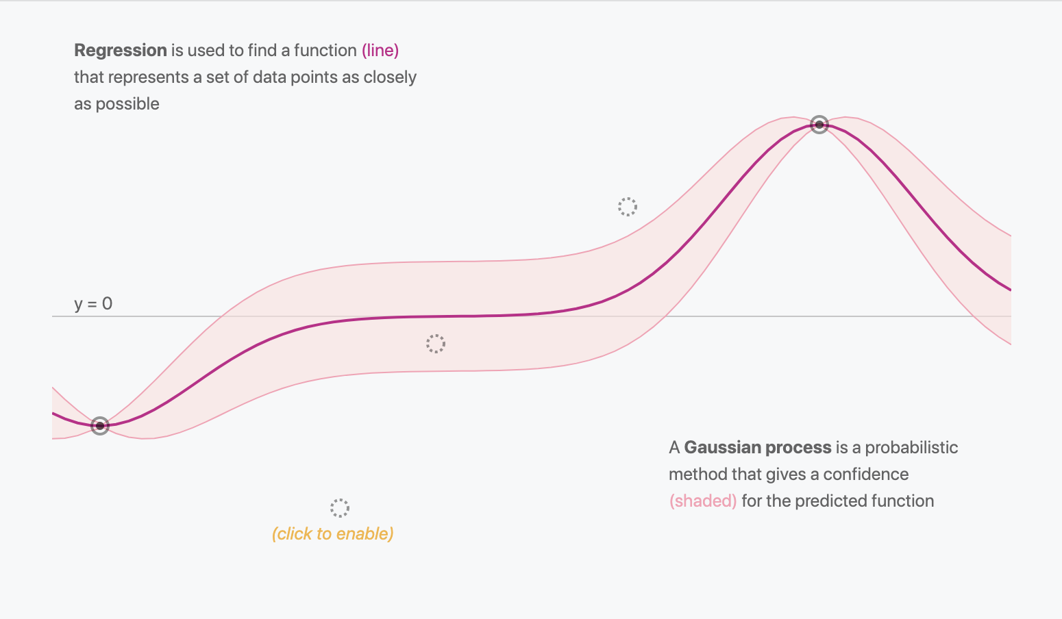
Gaussian Processes are a probabilistic framework for missing data imputation
a probabilistic imputation method - Advantages
Provides a framework to estimate values of missing data and their uncertainty
uncertainty will take into account how isolate the point is and how "predictable" (i.e. stationary) the process is
a probabilistic imputation method - Advantages
a probabilistic imputation method - Bayesian Framework
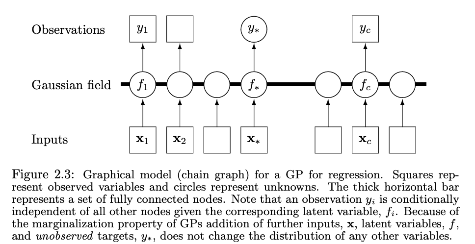
A process is a function i.e. something that can be calculated at any value of a (1- or N- dimensional) variable.
A process is a collection of random variables
a probabilistic imputation method - Bayesian Framework
A process is a function i.e. something that can be calculated at any value of a (1- or N- dimensional) variable.
A process is a collection of random variables
posterior
likelihood
prior
functions as fixed equations y=2x+3y=2x+3.
In GPs, we treat the function itself as a random variable. Instead of saying "the function is exactly this," we say "the function could be one of many possibilities, and here’s how likely each possibility is."
functions as fixed equations y=2x+3y=2x+3.
In GPs, we treat the function itself as a random variable. Instead of saying "the function is exactly this," we say "the function could be one of many possibilities, and here’s how likely each possibility is."
Gaussian Distribution:
For any set of input points (e.g., x1,x2,…,xnx1,x2,…,xn), the corresponding outputs (e.g., f(x1),f(x2),…,f(xn)f(x1),f(x2),…,f(xn)) are assumed to follow a joint Gaussian distribution.
A Gaussian Process is a specific type of process where:
Every finite collection of random variables is jointly Gaussian.
This means that if you pick any finite set of input points (e.g., x1,x2,…,xnx1, x2, ...xN) the corresponding predictions (y1, y2, yN) follow a multivariate Gaussian distribution.
functions as fixed equations y=2x+3y=2x+3.
In GPs, we treat the function itself as a random variable. Instead of saying "the function is exactly this," we say "the function could be one of many possibilities, and here’s how likely each possibility is."
Gaussian Distribution:
The probability of values generated by the processes is Gaussian at any point in the series (x-value).
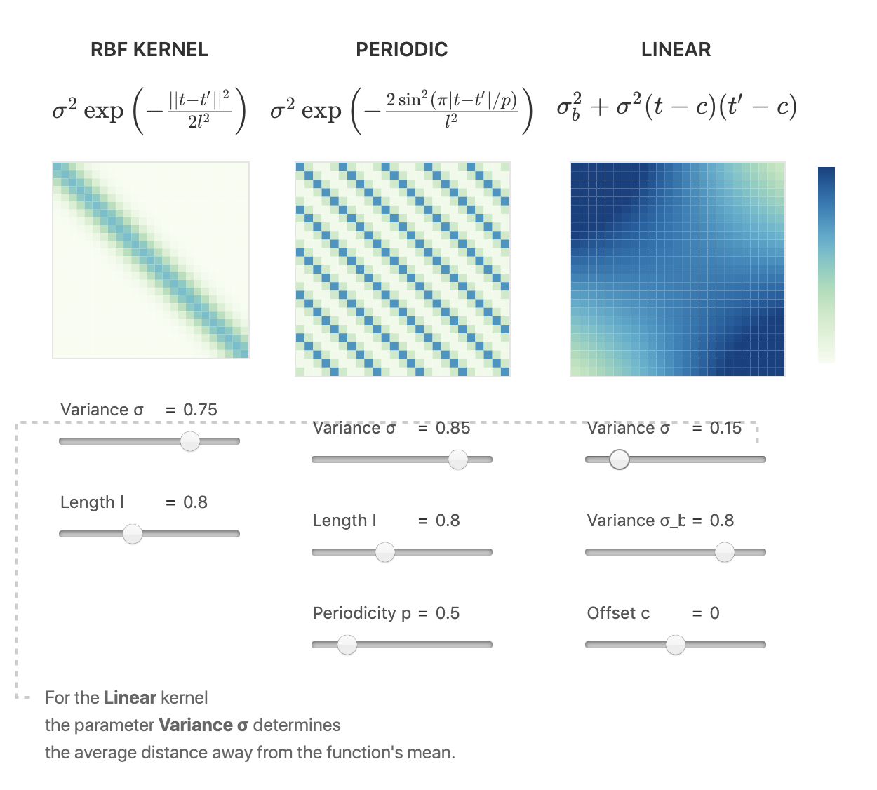
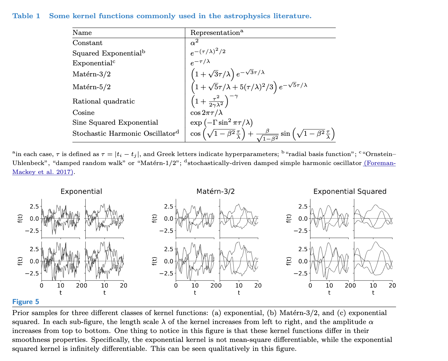
Kernel Function:
A kernel is a way to measure how similar two data points are. It tells the GP how much one point’s output should influence another point’s output. For example, if two points are close together, their outputs are likely to be similar.
A Gaussian Process is a specific type of process where:
Every finite collection of random variables is jointly Gaussian.
This means that if you pick any finite set of input points (e.g., x1,x2,…,xnx1, x2, ...xN) the corresponding predictions (y1, y2, yN) follow a multivariate Gaussian distribution.
A Gaussian Process is a specific type of process where:
The process is fully defined by a mean function and a covariance function.
The mean function describes the average behavior of the function.
The covariance function (kernel) describes how the function values at different input points are related.
a probabilistic imputation method - Applications
Prediction:
Predicting data based on the training set (this can naturally be done be in a regression but also in a classification context - GaussianProcess classifiers)
Like autoregressive models, it models y based on y (no context data)
a probabilistic imputation method - Bayesian Framework
Provides a framework to estimate values of missing data and their uncertainty
This is a Bayesian framework.
It is however NOT entirely a non-parametric method: you need to define a model (embedded in the kernel function, as we will see in a few slides)
The kernel is the prior
a probabilistic imputation method - Bayesian Framework
Probabilistic approach - Consider all possible functions but assign a prior to the ones that are more "likely"
Data imputation requires definition of a function:
a probabilistic imputation method - Advantages
It's computationally "tractable"
The framework defines an infinite set of "functions" that can be evaluated at each point: a single calculation provides the answer to the interpolation at any N points.
Each pair of function evaluations follows a bivariate Gaussian distribution
a probabilistic imputation method - Applications
Survey design:
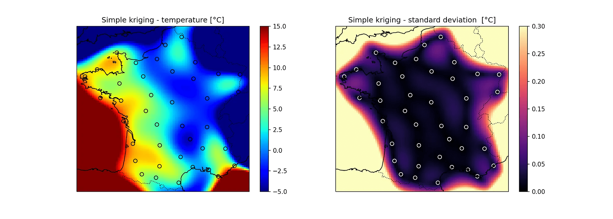
Identify where the uncertainty is largest to decide where to make observation (e.g. geospatial applications: where do I put my sensors?
Time domain: when to "mine" data from an existing but hard to access dataset.)
GP definitions
3.1
a probabilistic imputation method - Bayesian Framework
A process is a collection of random variables
A Gaussian processes is a collection of random variables any finite subset of which have joint Gaussian distribution.
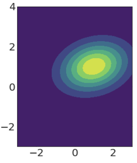
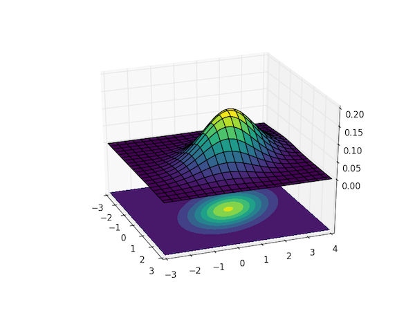
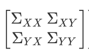
math: Multivariate Gaussian distributions
multivariate Gaussian distribution
μ: vector of means (expectation values)
σ: vector of standard deviation
Σ: matrix of covariance
Σ =
math: Multivariate Gaussian distributions
multivariate Gaussian distribution
μ: vector of means (expectation values)
σ: vector of standard deviation
Σ: matrix of covariance
Σ =
math: Multivariate Gaussian distributions
multivariate Gaussian distribution
μ: vector of means (expectation values)
σ: vector of standard deviation
Σ: matrix of covariance
Σ =
a probabilistic imputation method - Bayesian Framework
A Gaussian Process is entirely specified by its mean and covariance function.
The mean and covariance functions can be static or time-evolving
GP kernels
4
We predict each y(t) point based each other point in the time series and our prior believe about the points and their locations:
Define:
Kernels
Kernels
The Kernel is the prior distribution:
the kernel defines the consistency relation:
Kernels
The Kernel is the prior distribution:
kernels are functions (hence the method is parametric) and they have parameters that are learned
Kernels
The Kernel is the prior distribution:
(see kernel trick: the kernel allowed the solution to be found in a linear and therefore analytically solvable framework)
kernels are functions (hence the method is parametric) and they have parameters that are learned
Kernels
The Kernel is the prior distribution:
This says that we "believe" that the expectation of the values of y E[f(x)] =
e.g.
"double exponential kernel"
Kernels
The Kernel is the prior distribution:
e.g.
L: lag: distance between p and q
l: characteristic length
"double exponential kernel"
parameters
Kernels
This Kernel defines the mean.
With no observed data you can define a family of functions all pointwise distributes as a Gaussian around that mean
Kernels
This Kernel defines the mean.
With no observed data you can define a process, i.e., family of functions all pointwise distributes as a Gaussian around that mean
Each "process" is the P(y|t) posterior probability. The prior is the kernel, the likelihood is P(observed | y) where observed are the available data
P(Y) probability of the model (prior)
Kernels
As we include observations (the "training" data) the functions become limited to the functions that passes through (or near the data)
This Kernel defines the mean.
With no observed data you can define a process, i.e., family of functions all pointwise distributes as a Gaussian around that mean
Kernels
The Kernel also defines the posterior as a "similarity" function or as the memory of a time evolving process: how similar are points to each other? Including observed data
P(X |Y) probability of data given model
Kernels
At each t there is a Gaussian distributed family of y values
This Kernel defines the mean.
With no observed data you can define a process, i.e., family of functions all pointwise distributes as a Gaussian around that mean
Kernels
Kernels
Kernels
Kernels
the kernel defines the consistency relation of the Gaussian process:
Kernel
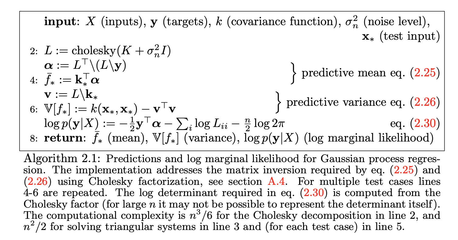
GP matrix formulation
4
Joint distribution or training and test data
Kernels
Joint distribution or training and test data
Kernels
assume the processes are mean 0. This is not necessary but simplified the math. Data can be preprocessed to be mean 0
Joint distribution or training and test data
Kernels
required matrix inversion
Joint distribution or training and test data, including uncertainties
Kernels
with independent observations and uncertainties with variance σ
Joint distribution or training and test data, including uncertainties
Kernels
with independent observations and uncertainties with variance σ
Kernels
Kernels
GP exercises
3
A Visual Exploration of Gaussian Processes
Jochen Görtler, Rebecca Kehlbeck, and Oliver Deussen
https://distill.pub/2019/visual-exploration-gaussian-processes/
Gaussian Processes for Machine Learning, the MIT Press
http://www.gaussianprocess.org/gpml/chapters/RW.pdf
its considered one of the best ML text ever written
A gentle introduction to Gaussian Process Regression
Dan Foreman Mackey - George user manual
SKlearn Gaussian Processes API manual
https://scikit-learn.org/stable/modules/gaussian_process.html
By federica bianco
Gaussian Processes


