


federica bianco PRO
astro | data science | data for good
Fall 2025 - UDel PHYS 641
dr. federica bianco
@fedhere
this slide deck:
1
Minkowski family of distances
Minkowski family of distances
Minkowski family of distances
N features (dimensions)
L1 is the Minkowski distance with p=1
L2 is the Minkowski distance with p=2 (Euclidean distance)
if p == infinity D(i,j)p ~ maxk (xik - xjk)
Minkowski family of distances
N features (dimensions)
properties:
Minkowski family of distances
Manhattan: p=1
features: x, y
Minkowski family of distances
Manhattan: p=1
features: x, y
Minkowski family of distances
Euclidean: p=2
features: x, y
2
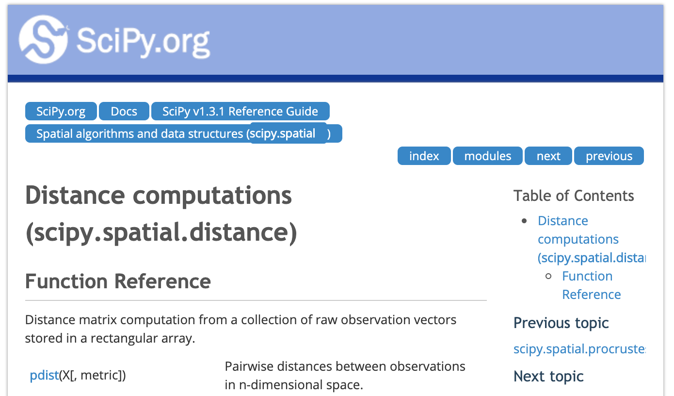
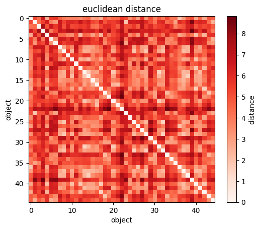
import scipy as sp

sp.spatial.distance.pdist(X) # the pairwise distance: returns (N**2  - N )/2 values for N objects

sp.spatial.distance.squareform(sp.spatial.distance.pdist(wines[["Alcohol", "Magnesium"]]))
#returns the NXN matrix of distances

plt.imshow(sp.spatial.distance.squareform(sp.spatial.distance.pdist(wines[["Alcohol", "Magnesium"]])))
#you can visualize the NXN matrix


plt.xlabel("wine")
plt.ylabel("wine");
plt.colorbar(label="distance");
import scipy as sp
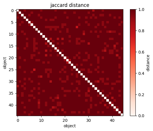
sp.spatial.distance.pdist(X) # the pairwise distance: returns (N**2 - N )/2 values for N objects
sp.spatial.distance.squareform(sp.spatial.distance.pdist(wines[["Alcohol", "Magnesium"]],
metric='jaccard'))
#returns the NXN matrix of distances
plt.imshow(sp.spatial.distance.squareform(sp.spatial.distance.pdist(wines[["Alcohol", "Magnesium"]])))
#you can visualize the NXN matrix
plt.xlabel("wine")
plt.ylabel("wine");
plt.colorbar(label="distance");Siddarth Chiaini, UDelaware
3
classification
prediction
feature selection
supervised learning
understanding structure
organizing/compressing data
anomaly detection dimensionality reduction
unsupervised learning
classification
supervised learning methods
(nearly all other methods you heard of)
learns by example
used to:
classify, predict (regression)
x
y
observed features:
(x, y)
models typically return a partition of the space
goal is to partition the space so that the unobserved variables are
separated in groups
consistently with
an observed subset
target features:
(color)
x
y
observed features:
(x, y)
if x**2 + y**2 <= (x-a)**2 + (y-b)**2 :
	return blue
else:
	return orange
target features:
(color)
A subset of variables has class labels. Guess the label for the other variables
SVM
finds a hyperplane that optimally separates observations
x
y
observed features:
(x, y)
Tree Methods
split spaces along each axis separately
A subset of variables has class labels. Guess the label for the other variables
split along x
if x <= a :
	if y <= b:
      		return blue
return orange
then
along y
target features:
(color)
x
y
observed features:
(x, y)
KNearest Neighbors
Assigns the class of closest neighbors
A subset of variables has class labels. Guess the label for the other variables
if (labels[argmin(distance((x,y), trainingset))][:4] == blue)sum() > (labels[argmin(distance((x,y), trainingset))][:4] == orange)sum():
	return blue
return orange
target features:
(color)
Calculate the distance d to all known objects

Select the k closest objects

Assign the most common among the k classes:
# k = 1
d = distance(x, trainingset)
C(x) = C(trainingset[argmin(d)])
Calculate the distance d to all known objects

Select the k closest objects
Classification:
Assign the most common among the k classes
Regression:
Predict the average (median) of the k target values
Good
non parametric
very good with large training sets
Cover and Hart 1967: As n→∞, the 1-NN error is no more than twice the error of the Bayes Optimal classifier.
Good
non parametric
very good with large training sets
Cover and Hart 1967: As n→∞, the 1-NN error is no more than twice the error of the Bayes Optimal classifier.
Let xNN be the nearest neighbor of x.
For n→∞, xNN→x(t) => dist(xNN,x(t))→0
Theorem: e[C(x(t)) = C(xNN)]< e_BayesOpt
e_BayesOpt = argmaxy P(y|x)
Proof: assume P(y|xt) = P(y|xNN)
(always assumed in ML)
eNN = P(y|x(t)) (1−P(y|xNN)) + P(y|xNN) (1−P(y|x(t))) ≤
(1−P(y|xNN)) + (1−P(y|x(t))) =
2 (1−P(y|x(t)) = 2ϵBayesOpt,
Good
non parametric
very good with large training sets
Not so good
it is only as good as the distance metric
If the similarity in feature space reflect similarity in label then it is perfect!
poor if training sample is sparse
poor with outliers
dynamic programming
4
Breaking down a problem into subproblems
Solve the subproblem once and store the solution
Instead of recomputing look up the solution as needed
Trade off: decreases computational complexity (commonly exponential problems O(exp(n)) are solvable in quadratic time O(n^2) or O(n^3)
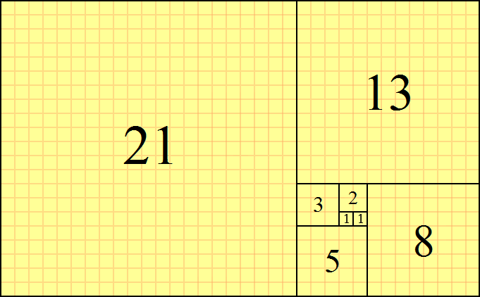
Example: Fibonacci sequency
# function recursively called
def fib (n) :
  if (n < 2):
    return n
  return fib(n-1) + fib(n-2)
# dynamin programming approach
def fibDP (n) :
fibresult = np.zeros(n+1, int)
fibresult[1] = 1
for i in np.arange(2, n+1):
fibresult[i] = fibresult[i-1] + fibresult[i-2]
return fibresult[-1]0, 1, 1, 2, 3, 5, 8, 13, 21, 34, 55, 89, 144, ...
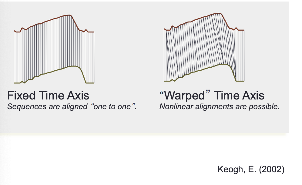
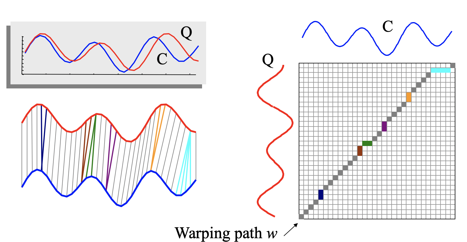
Dynamic time warping
5
Sakoe & Chiba 1978
Row-feature methods are very sensitives to "irrelevant" differences
1D
2D
x
y
2D
| X | Y | |
|---|---|---|
| A | x1 | y1 |
| B | x2 | y2 |
y2
y1
x1
x2
x
y
A B
x1
x2
x3
x4
x5
x6
scipy.spatial.distance_matrix(np.atleast_2d(A).T, np.atleast_2d(B).T)
A B
x1
x2
x3
x4
x5
x6
scipy.spatial.distance_matrix(np.atleast_2d(A).T, np.atleast_2d(B).T)
x1
x2
x3
x4
x5
x6
A-x1
B-x4
A-x1
np.sqrt((np.diag(scipy.spatial.distance_matrix(np.atleast_2d(A).T, np.atleast_2d(B).T))**2).sum())scipy.spatial.distance_matrix(np.atleast_2d(A).T, np.atleast_2d(B).T)
x1
x2
x3
x4
x5
x6
np.sqrt((np.diag(scipy.spatial.distance_matrix(np.atleast_2d(A).T, np.atleast_2d(B).T))**2).sum())A B
x1
x2
x3
x4
x5
x6
A B
x1
x2
x3
x4
x5
x6
D
121
91
64
121
126
121
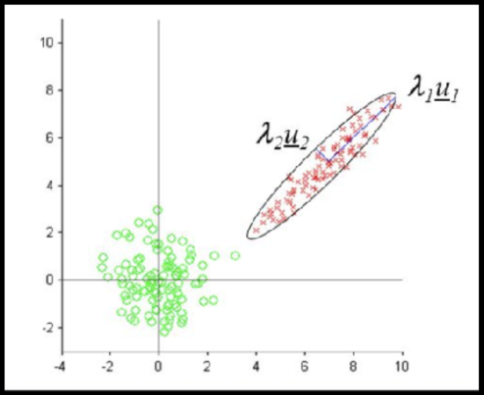
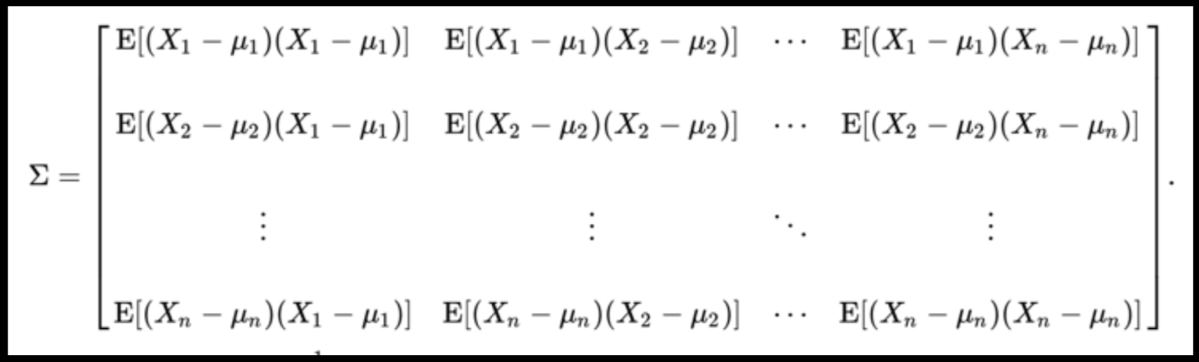
Data that is not correlated appear as a sphere in the Ndimensional feature space
Data can have covariance (and it almost always does!)
ORIGINAL DATA
STANDARDIZED DATA
Generic preprocessing
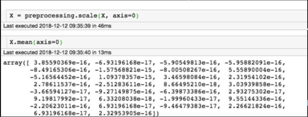
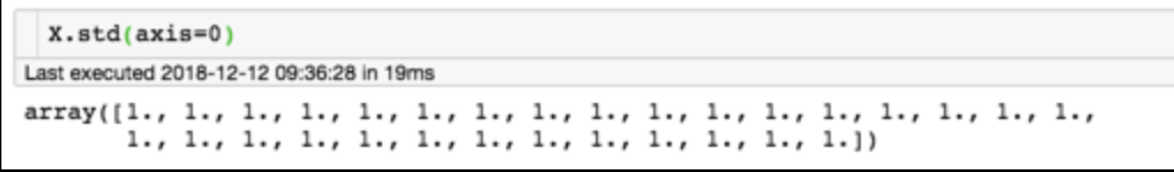
When standardizing a dataset we take every features and we force them to be the mean=0 standard deviation=1
Generic preprocessing
for each feature: divide by standard deviation and subtract mean
mean of each feature should be 0, standard deviation of each feature should be 1
Generic preprocessing
for each feature: divide by standard deviation and subtract mean
mean of each feature should be 0, standard deviation of each feature should be 1
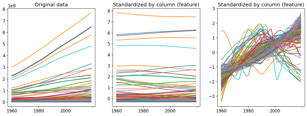
Time Series Preprocessing
what happens if I standardize a dataset by time stamp??
mean of each feature should be 0, standard deviation of each ROW (time series) should be 1
That way we compare shapes of time series, i.e. trends!
D
D
D
| t1 | t2 | t3 | t4 | t5 | t6 | |
|---|---|---|---|---|---|---|
| obs1 | 6.5 | 8.5 | 6.2 | 9.9 | 5.5 | 8.5 |
| obs2 | 0.0 | 1.0 | -0.1 | 1.9 | -0.5 | 1.0 |
μ=0, σ=1
μ=0, σ=1
x1
D
PREPROCESSING TIME SERIES
7.5
0
timeSeriesScaled = sklearn.preprocessing.scale(timeSeries, axis=1, with_std=False)
Generally I am interested in a similar shape. If I were interested in the absolute distance I would be better off with feature extraction!
| t1 | t2 | t3 | t4 | t5 | t6 | |
|---|---|---|---|---|---|---|
| obs1 | 6.5 | 8.5 | 6.2 | 9.9 | 5.5 | 8.5 |
| obs2 | -0.6 | 0.6 | -0.8 | 1.5 | -1.2 | 0.6 |
μ=0, σ=1
μ=0, σ=1
x1
D
PREPROCESSING TIME SERIES
0
0
timeSeriesScaled = sklearn.preprocessing.scale(timeSeries, axis=1, with_std=False)
Generally I am interested in a similar shape. If I were interested in the absolute distance I would be better off with feature extraction!
| t1 | t2 | t3 | t4 | t5 | t6 | |
|---|---|---|---|---|---|---|
| obs1 | -1.0 | 1.0 | 1.3 | 2.4 | 2.0 | 1.0 |
| obs2 | -0.6 | 0.6 | -0.8 | 1.5 | -1.2 | 0.6 |
μ=0, σ=1
μ=0, σ=1
D
PREPROCESSING TIME SERIES
0
0
timeSeriesScaled = sklearn.preprocessing.scale(timeSeries, axis=1)
Generally I am interested in a similar shape. If I were interested in the absolute distance I would be better off with feature extraction!
| t1 | t2 | t3 | t4 | t5 | t6 | |
|---|---|---|---|---|---|---|
| obs1 | -0.6 | 0.6 | 0.8 | 1.5 | -1.2 | 0.6 |
| obs2 | -0.6 | 0.6 | -0.8 | 1.5 | -1.2 | 0.6 |
μ=0, σ=1
μ=0, σ=1
Standardizing (scaling)
assures we are measuring similarity in shape, regardless of absolute numbers
0
0
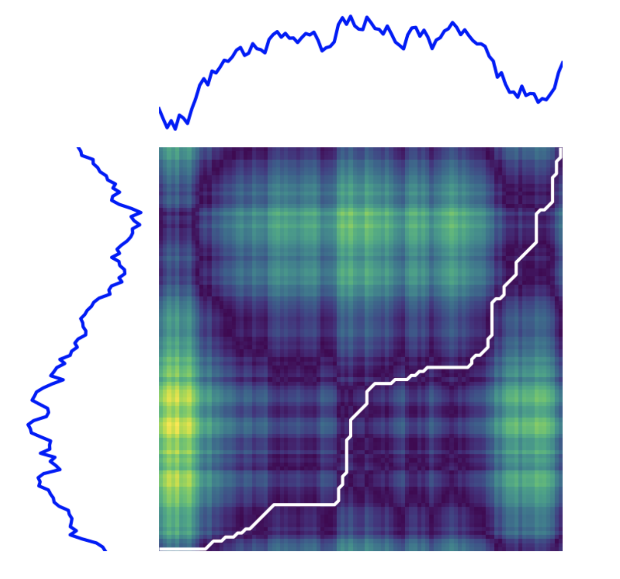
Time Warped time series
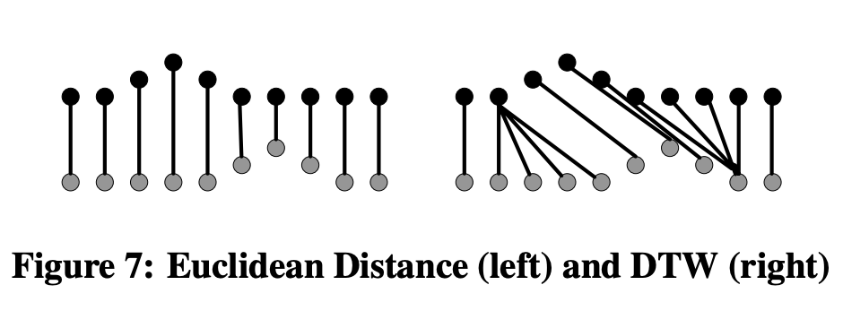
A warping of the time axis would also suppress similarity
The first plot (left) corresponds to measuring the distance along each axis and combine those distances (e.g. Eucledian)
The right plot is how we deal with "time warping"
Modify the distance matrix by considering the points surrounding the diagonal
|
0 |
|||||
|---|---|---|---|---|---|
|
0 |
|||||
|
0 |
d(Qi-1,Qj) | ||||
| d(Qi,Qj-1) |
0 |
||||
|
0 |
|||||
|
0 |
x1
x2
x3
x4
x5
x6
x1
x2
x3
x4
x5
x6
x1
x6
Modify the distance matrix by considering the points surrounding the diagonal
|
0 |
|||||
|
0 |
|||||
|
0 |
d(Qi,Qi+1) | ||||
| d(Qi+i,Qi) |
0 |
||||
|
0 |
|||||
|
0 |
x1
x2
x3
x4
x5
x6
x1
x2
x3
x4
x5
x6
x1
x6
Modify the distance matrix by considering the points surrounding the diagonal
x1
x2
x3
x4
x5
x6
x1
x2
x3
x4
x5
x6
x1
x6
|
0 |
|||||
|
0 |
|||||
|
0 |
d(Qi,Qi+1) | ||||
| d(Qi+i,Qi) |
0 |
||||
|
0 |
|||||
|
0 |
Modify the distance matrix by considering the points surrounding the diagonal
| d(Q0, C0) | |||||
|---|---|---|---|---|---|
| d(Qi-1,Ci-1) | d(Qi-1,Ci) | ||||
| d(Qi, Ci-1) | d(Qi, Ci) | ||||
| d(Qn, Cn) |
- first step is always d(Q0,C0)
- if distance is smaller you may deviate off the diagonal
DTW(Qi, Cj) = d(Qi, Cj) + min(d(Qi-1, Ci-1), d(Qi-1, Cj), d(Qi, Cj-1))
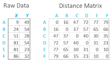
To align two sequences using DTW, an n-by-n matrix is constructed, with the (ith, jth) element of the matrix being the Euclidean distance
d(qi, cj) between the points qi and cj .
DTW(Qi, Cj) = d(Qi, Cj) + min(d(Qi-1, Ci-1), d(Qi-1, Cj), d(Qi, Cj-1))
To align two sequences using DTW, an n-by-n matrix is constructed, with the (ith, jth) element of the matrix being the Euclidean distance
d(qi, cj) between the points qi and cj .
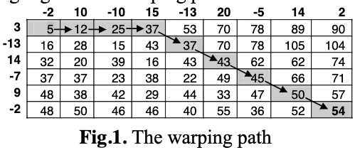
A warping path P is a contiguous set of matrix elements that defines a mapping between Q and C. The tth element of P is defined as pt=(i, j)t :
P = p1, p2, …, pt,
n ≤ T ≤ 2n-1
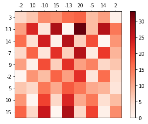
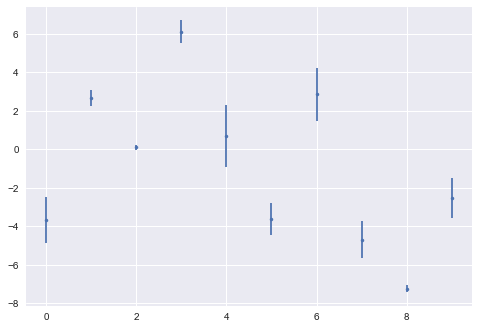
import numpy as np
import pylab as pl
import scipy as sp
x = np.array([-2, 10, -10, 15, 13, 20, 5, 14, 2])
y = np.array([3, -13, 14, -7, 9, 20, -2, 14, 2])

distm = sp.spatial.distance_matrix(x.reshape(-1,1),
                           y.reshape(-1,1), p=1)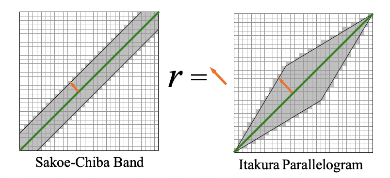
pl.imshow(distm)r is the parameter of serach
DTW(Qi, Cj) = d(Qi, Cj) + min(d(Qi-1, Ci-1), d(Qi-1, Cj), d(Qi, Cj-1))
Sakoe & Chiba 78
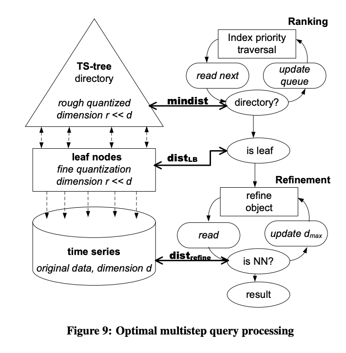
Indexing time series
6
“…we have about a million samples per minute coming in from 1000 gas turbines around the world… we need to be able to do similarity search for...” Lane Desborough, GE. • “…an archival rate of 3.6 billion points a day, how can we (do similarity search) in this data?” Josh Patterson, TVA. Our
iSAX 2.0: Indexing and Mining One Billion Time Series
We show that the main bottleneck in mining such massive datasets is the time taken to build the index
indexing refers to organizing observations (here a time series is an observation) so that they can be searched.
Indexing is at the root of databasing
iSAX 2.0: Indexing and Mining One Billion Time Series
We show that the main bottleneck in mining such massive datasets is the time taken to build the index
t = (t1, . . . , tn), ti ∈ R,
where time point f(i) is before f(i + 1):
f(i) < f(i + 1),
and f : N → R is a function mapping indices to time points.
Long time series data which is treated as point data, corresponds to very high dimensional feature spaces.
t = (t1, . . . , tn), ti ∈ R,
where time point f(i) is before f(i + 1):
f(i) < f(i + 1),
and f : N → R is a function mapping indices to time points.
Long time series data which is treated as point data, corresponds to very high dimensional feature spaces.
Indexing create a compact yet detailed index structure for time series similarity search and retrieval.
storage efficient
indexing is about finding compact representations that allow to simplify the search problem: so that you do not habve to measure the distance between all time series
indexing is about finding compact representations that allow to simplify the search problem: so that you do not habve to measure the distance between all time series
Effective DTW models
6
A time series of length one trillion is a very large data object. In
fact, it is more than all of the time series data considered in all
papers ever published in all data mining conferences combined.
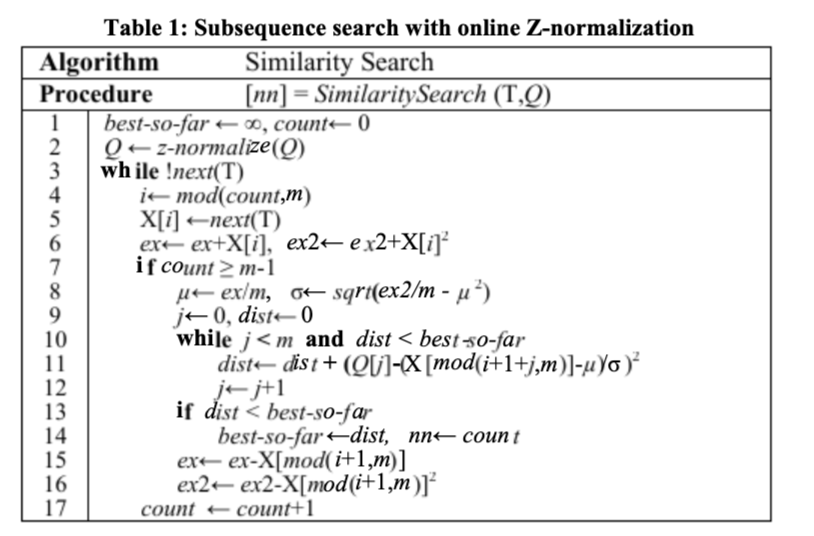
1 Time Series Subsequences must be Normalized
2 Arbitrary Query Lengths cannot be Indexed
If we know the length of queries ahead of time we can mitigate at least some of the intractability of search by indexing the data. Although to our knowledge no one has built an index for a trillion real-valued objects (Google only indexed a trillion webpages as recently as 2008), perhaps this could be done.
4.1.1 Using the Squared Distance
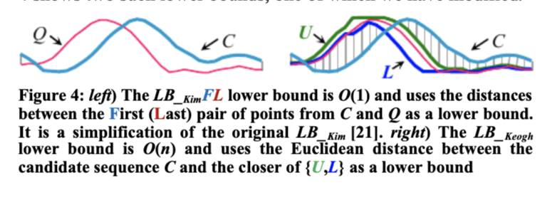
4.1.2 Lower Bounding (LB_keog)
4.1.3 Early Abandoning of ED and LB_keog
4.1.4 Early Abandoning of DTW
4.1.1 Using the Squared Distance
4.1.2 Lower Bounding (LB_keog)
4.1.3 Early Abandoning of ED and LB_keog
4.1.4 Early Abandoning of DTW
4.1.1 Using the Squared Distance
4.1.2 Lower Bounding (LB_keog)
4.1.3 Early Abandoning of ED and LB_keog
4.1.4 Early Abandoning of DTW
if we note that the current metric
differences between each pair of corresponding datapoints
exceeds the best-so-far we abandon
4.2.1 Early Abandoning Z-Normalization
this step is heavily relying on dynamic programming
4.2.1 Early Abandoning Z-Normalization
4.2.2 Reordering Early Abandoning
4.2.3 Reversing the Query/Data Role in LB
4.2.4 Cascading Lower Bounds
universal optimal ordering that we can
compute in advance:
The sections of the query
that are farthest from the mean, zero, will on average have the
largest contributions to the distance measure.
4.1.1 Using the Squared Distance
4.1.2 Lower Bounding (LB_keog)
4.1.3 Early Abandoning of ED and LB_keog
4.1.4 Early Abandoning of DTW
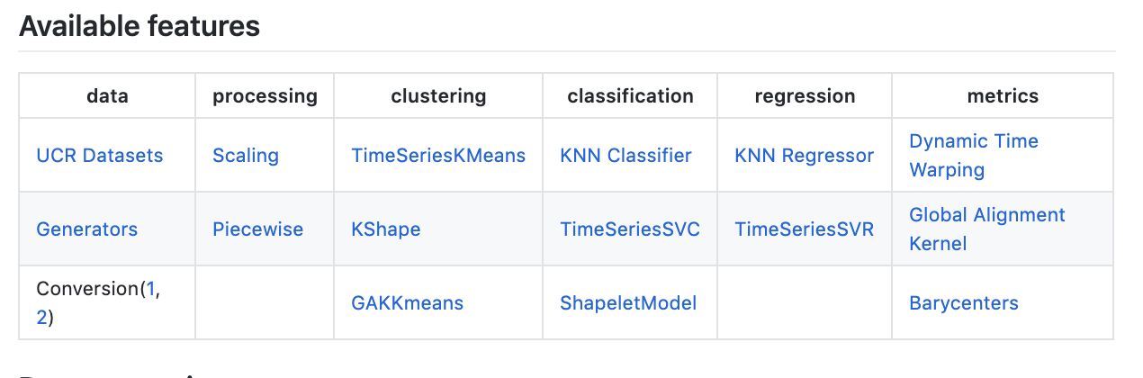
Python DTW implementation
7
from tslearn.preprocessing import TimeSeriesScalerMeanVariance
from tslearn import metrics
scaler = TimeSeriesScalerMeanVariance(mu=0., std=1.)  # Rescale
dataset_scaled = scaler.fit_transform(dataset)

path, sim = metrics.dtw_path(dataset_scaled[0], dataset_scaled[1])
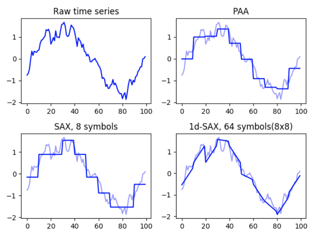
from tslearn.preprocessing import TimeSeriesScalerMeanVariance
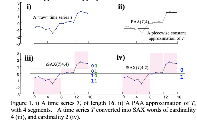
from tslearn.piecewise import PiecewiseAggregateApproximation
scaler = TimeSeriesScalerMeanVariance(mu=0., std=1.) # Rescale
dataset = scaler.fit_transform(dataset)
# PAA transform (and inverse transform) of the data
n_paa_segments = 10
paa = PiecewiseAggregateApproximation(n_segments=n_paa_segments)
paa_dataset_inv = paa.inverse_transform(paa.fit_transform(dataset))use for feature engineering!
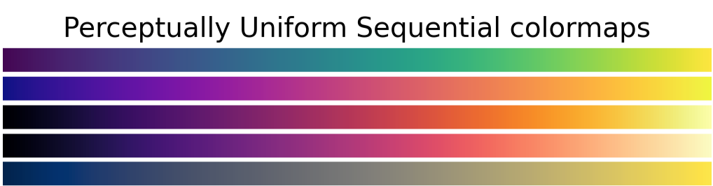
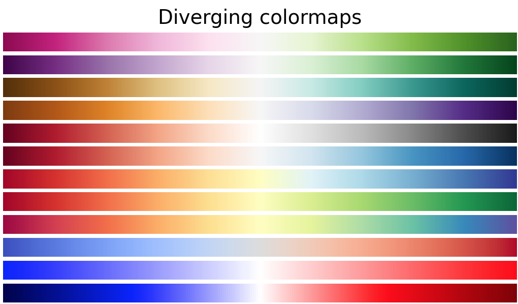
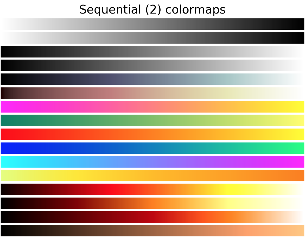
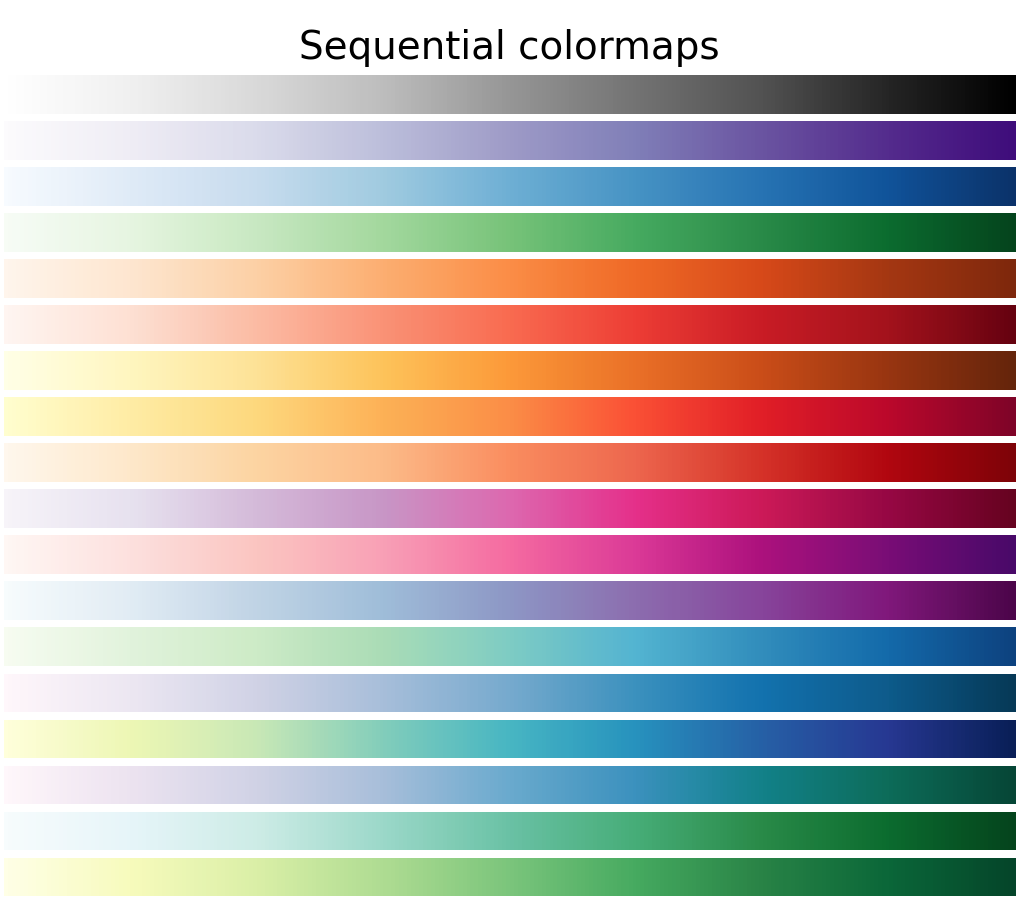
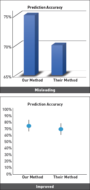
visualization tips: color maps
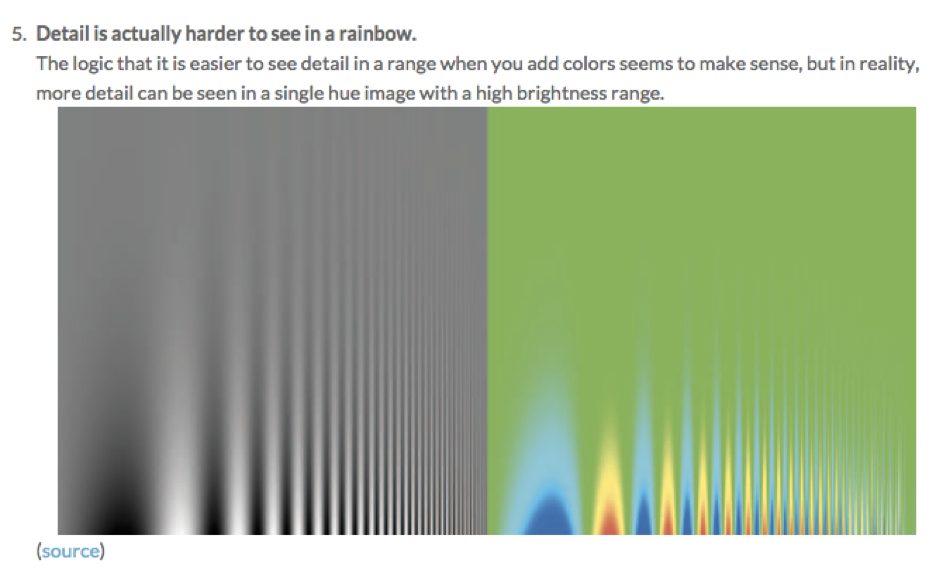
Color maps that are perceptually homogeneous respect relationships between data
data-ink ratio (Edward Tufte)
Dynamic Programming Algorithm Optimization for
Spoken Word Recognition Sakoe & Chiba 1978 (original DTW paper)
Exact indexing of dynamic time warping
Eamonn Keogh, Chotirat Ann Ratanamahatana 2002 (slides)
https://www.cs.ucr.edu/~eamonn/KAIS_2004_warping.pdf
Searching and Mining Trillions of Time Series Subsequences under Dynamic Time Warping
Rakthanmanon et al 2012 (computational aspect of DTW)
Querying and Mining of Time Series Data: Experimental Comparison of Representations and Distance Measures
Hui Ding Goce Trajcevski Peter Scheuermann Xiaoyue Wang & Eamonn Keogh
https://www.cs.ucr.edu/~eamonn/vldb_08_Experimental_comparison_time_series.pdf
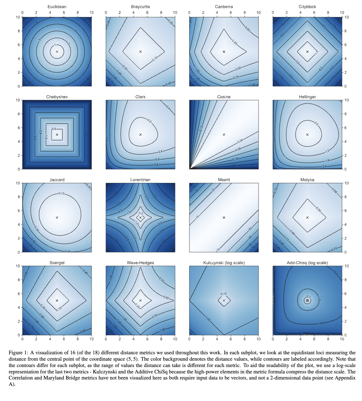
you must be able tp describe in general all of figures 7-13 and in detail one of those figures.
code up the DTW algorithm and apply it to sound bites, find the notebook in https://github.com/fedhere/MLTSA_FBianco/tree/master/HW7
code up the DTW algorithm and apply it to sound bites, find the notebook in https://github.com/fedhere/MLTSA_FBianco/tree/master/HW7
def path(matrix):
	# the path can be calculated backword or forward
	# I find bacward more intuitive
	# start at one to the last cell:
	i, j = list(matrix.shape - 2)
    #since I do not know how long the path is i will use lists
    # p and q will be the list of indices of the path element along the 2 array axes
    p, q = [i], [j]
    # go all the way to cell 0,0
    while (i > 0) or (j > 0):
      	# pick minimum of 3 surrounding elements:
      	# the diagonal and the 2 surrounding it
        tb = argmin((D[i, j], D[i, j + 1], D[i + 1, j]))
        #stay on the diagonal
        if tb == 0:
            i -= 1
            j -= 1
        #off diagonal choices: move only up or sideways
        elif tb == 1:
            i -= 1
        else:  # (tb == 2):
            j -= 1
        # put i and the j indexx into p and q pushing existing entries forward
        p.insert(0, i)
        q.insert(0, j)
    return array(p), array(q)
code to calculate
the path
along the DTW array
for plotting
classification
prediction
feature selection
supervised learning
understanding structure
organizing/compressing data
anomaly detection dimensionality reduction
unsupervised learning
understand structure of feature space
prediction based on examples (inferential AI)
generate new instances (generative AI)
=> second order purpose | feature importance
[Machine Learning is the] field of study that gives computers the ability to learn without being explicitly programmed. Arthur Samuel, 1959
model
parameters:
slope, intercept
data
ML: any model with parameters learnt from the data
[Machine Learning is the] field of study that gives computers the ability to learn without being explicitly programmed. Arthur Samuel, 1959
model
parameters:
slope, intercept
data
ML: any model with parameters learnt from the data
Via minimization of a loss function
Loss function is "distance" between known and predicted values of the target variable
supervised learning
????
unsupervised learning
why
understand structure of feature space
- dimensionality reduction
- anomaly detection
(e.g. image compression)
ML model have parameters and hyperparameters
parameters: the model optimizes based on the data
hyperparameters: chosen by the model author, could be based on domain knowledge, other data, guessed (?!).
e.g. the shape of the polynomial
observed features:
(x, y)
GOAL: partitioning data in maximally homogeneous,
maximally distinguished subsets.
x
y
all features are observed for all objects in the sample
(x, y)
how should I group the observations in this feature space?
e.g.: how many groups should I make?
x
y
internal criterion:
members of the cluster should be similar to each other (intra cluster compactness)
external criterion:
objects outside the cluster should be dissimilar from the objects inside the cluster
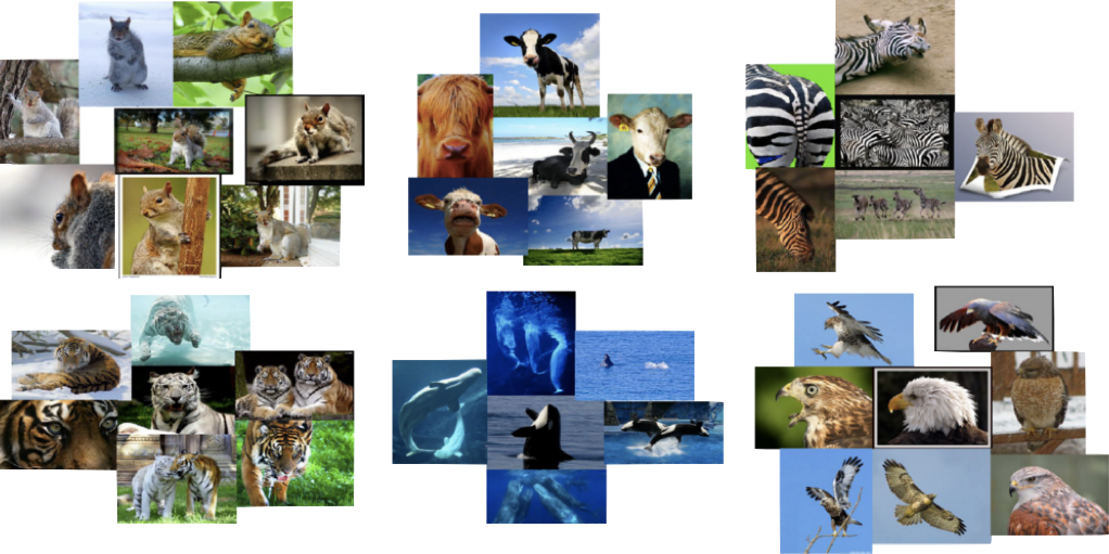
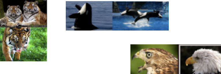
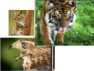
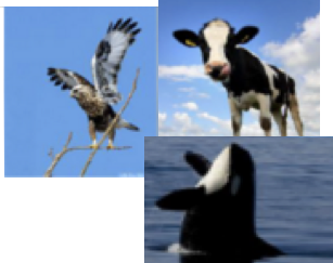
tigers
wales
raptors
zoologist's clusters
orange/green
black/white/blue
internal criterion:
members of the cluster should be similar to each other (intra cluster compactness)
external criterion:
objects outside the cluster should be dissimilar from the objects inside the cluster
photographer's clusters
how you define similarity/distance
internal criterion:
members of the cluster should be similar to each other (intra cluster compactness)
external criterion:
objects outside the cluster should be dissimilar from the objects inside the cluster
Scalability (naive algorithms are Np hard)
Ability to deal with different types of attributes
Discovery of clusters with arbitrary shapes
Minimal requirement for domain knowledge
Deals with noise and outliers
Insensitive to order
Allows incorporation of constraints
Interpretable
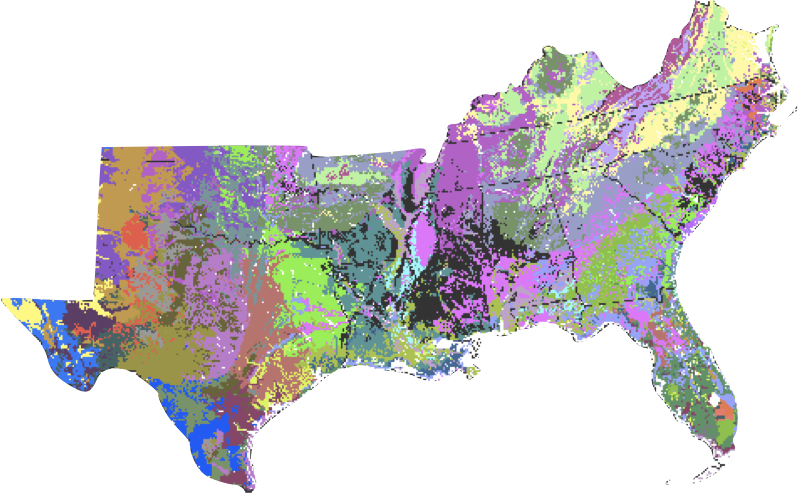
A Spatial Clustering Technique for the Identification of Customizable Ecoregions
William W. Hargrove and Robert J. Luxmoore
50-year mean monthly temperature, 50-year mean monthly precipitation, elevation, total plant-available water content of soil, total organic matter in soil, and total Kjeldahl soil nitrogen
THIS CLUSTERING IS NOT BASED ON LOCATION! but on properties of the location that have a spatial coherence
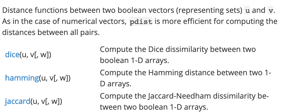
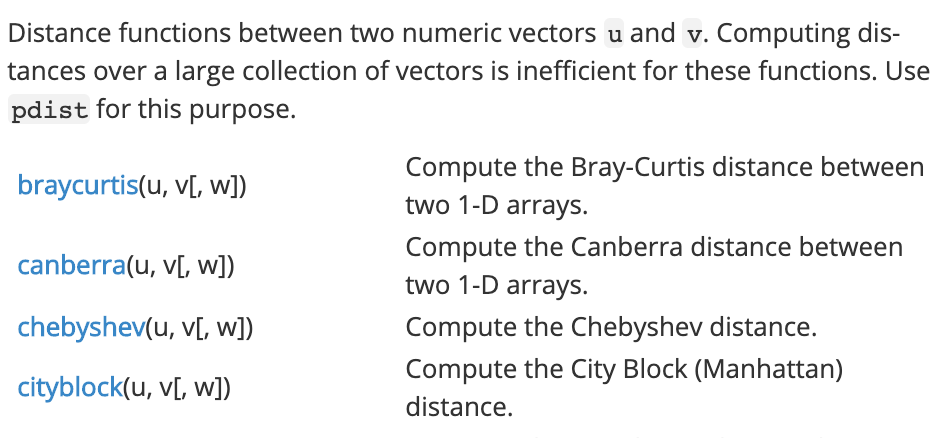
We already cover and reviewed distances for continuous variables. Briefly lets look at categorical distances:
Uses presence/absence of features in data
: number of features in neither
: number of features in both
: number of features in i but not j
: number of features in j but not i
What is the distance between a leopard and a lizard?
- they both have tails
- only lizards have scales
- neither have wings
Uses presence/absence of features in data
: number of features in neither
: number of features in both
: number of features in i but not j
: number of features in j but not i
What is the distance between a leopard and a lizard?
- they both have tails
- only lizards have scales
- neither have wings
| 1 | 0 | sum | |
|---|---|---|---|
| 1 | M11 | M10 | M11+M10 |
| 0 | M01 | M00 | M01+M00 |
| sum | M11+M01 | M10+M00 | M11+M00+M01+ M10 |
observation i
}
}
| 0 | sum | ||
|---|---|---|---|
| 1 | M10 | M11+M10 | |
| 0 | M01 | M00 | M01+M00 |
| sum | M11+M01 | M10+M00 | M11+M00+M01+ M10 |
1
1
1
0
observation j
Uses presence/absence of features in data
: number of features in neither
: number of features in both
: number of features in i but not j
: number of features in j but not i
What is the distance between a leopard and a lizard?
- they both have tails
- only lizards have scales
- neither have wings
| 1 | 0 | sum | |
|---|---|---|---|
| 1 | M11 | M10 | M11+M10 |
| 0 | M01 | M00 | M01+M00 |
| sum | M11+M01 | M10+M00 | M11+M00+M01+ M10 |
observation i
}
}
| 0 | sum | ||
|---|---|---|---|
| 1 | M10 | M11+M10 | |
| 0 | M01 | M00 | M01+M00 |
| sum | M11+M01 | M10+M00 | M11+M00+M01+ M10 |
observation j
Simple Matching Distance
Uses presence/absence of features in data
Simple Matching Coefficient
or Rand similarity
| 1 | 0 | sum | |
|---|---|---|---|
| 1 | M11 | M10 | M11+M10 |
| 0 | M01 | M00 | M01+M00 |
| sum | M11+M01 | M10+M00 | M11+M00+M01+ M10 |
observation i
observation j
}
}
| 0 | sum | ||
|---|---|---|---|
| 1 | M11 | M10 | M11+M10 |
| 0 | M01 | M00 | M01+M00 |
| sum | M11+M01 | M10+M00 | M11+M00+M01+ M10 |
lizard/leopard
1
1
1
0
Jaccard similarity
Jaccard distance
| 1 | 0 | sum | |
|---|---|---|---|
| 1 | M11 | M10 | M11+M10 |
| 0 | M01 | M00 | M01+M00 |
| sum | M11+M01 | M10+M00 | M11+M00+M01+ M10 |
observation i
observation j
}
}
lizard/leopard
Jaccard similarity
Jaccard distance
| 1 | 0 | sum | |
|---|---|---|---|
| 1 | M11 | M10 | M11+M10 |
| 0 | M01 | M00 | M01+M00 |
| sum | M11+M01 | M10+M00 | M11+M00+M01+ M10 |
observation i
observation j
}
}
Jaccard similarity
Application to Deep Learning for image recognition
Convolutional Neural Nets
K-means (McQueen ’67)
K-medoids (Kaufman & Rausseeuw ’87)
Expectation Maximization (Dempster,Laird,Rubin ’77)
Hard partitioning cluster method
Choose N “centers” guesses: random points in the feature space
repeat:
  Calculate distance between each point and each center

  Assign each point to the closest center

  Calculate the new cluster centers

untill (convergence):
  when clusters no longer change
Objective: minimizing the aggregate distance within the cluster.
Order: #clusters #dimensions #iterations #datapoints O(KdN)
CONs:
Its non-deterministic: the result depends on the (random) starting point
It only works where the mean is defined: alternative is K-medoids which represents the cluster by its central member (median), rather than by the mean
Must declare the number of clusters upfront (how would you know it?)
PROs:
Scales linearly with d and N
Objective: minimizing the aggregate distance within the cluster.
Order: #clusters #dimensions #iterations #datapoints O(KdN)
O(KdN):
complexity scales linearly with
-d number of dimensions
-N number of datapoints
-K number of clusters
either you know it because of domain knowledge
or
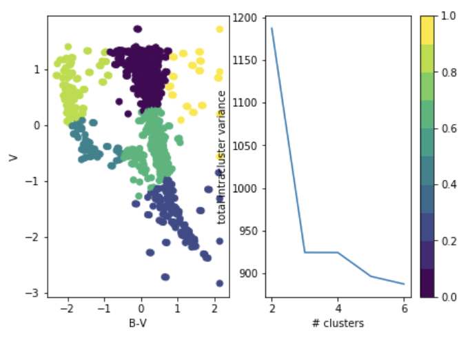
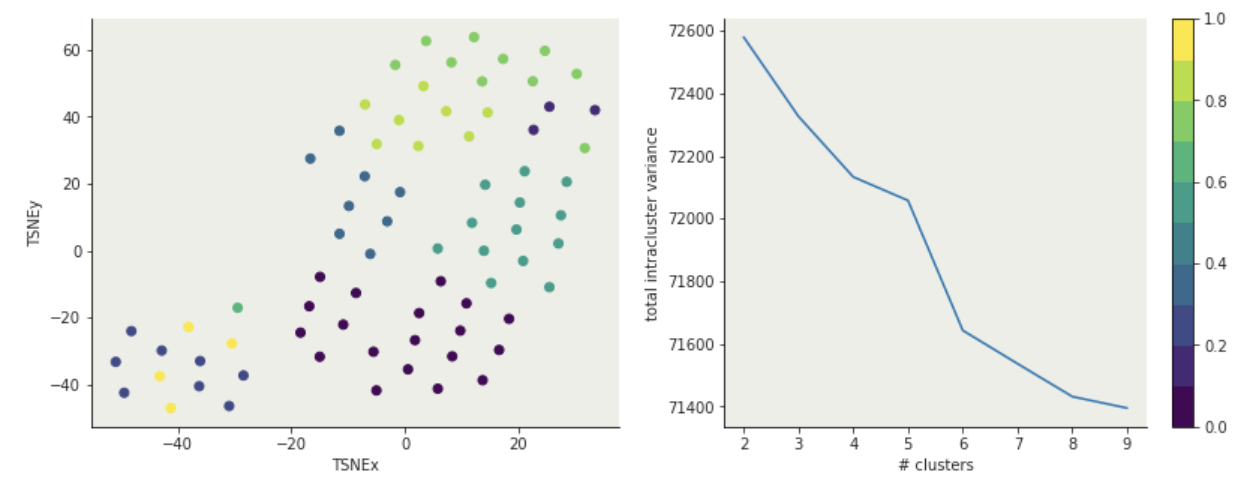
you choose it after the fact: "elbow method"
total intra-cluster variance
Objective: minimizing the aggregate distance within the cluster.
Order: #clusters #dimensions #iterations #datapoints O(KdN)
Must declare the number of clusters
Objective: minimizing the aggregate distance within the cluster.
Order: #clusters #dimensions #iterations #datapoints O(KdN)
Must declare the number of clusters upfront (how would you know it?)
either domain knowledge or
after the fact: "elbow method"
total intra-cluster variance
‘k-means++’ : selects initial cluster centers for k-mean clustering in a smart way to speed up convergence. See section Notes in k_init for more details.
‘random’: choose k observations (rows) at random from data for the initial centroids.
If an ndarray is passed, it should be of shape (n_clusters, n_features) and gives the initial centers.
Convergence Criteria
General
Any time you have an objective function (or loss function) you need to set up a tolerance : if your objective function did not change by more than ε since the last step you have reached convergence (i.e. you are satisfied)
ε is your tolerance
For clustering:
convergence can be reached if
no more than n data point changed cluster
n is your tolerance
Soft partitioning cluster method
Hard clustering : each object in the sample belongs to only 1 cluster
Soft clustering : to each object in the sample we assign a degree of belief that it belongs to a cluster
Soft = probabilistic
SKIP IN CLASS BUT YOU CAN LOOK AT THE SLIDES ON YOUR OWN!!
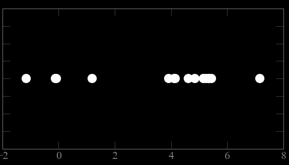
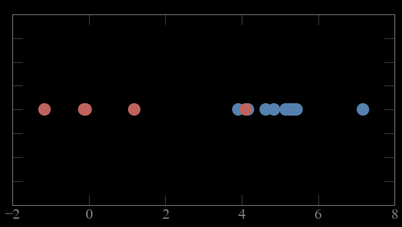
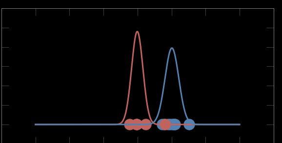
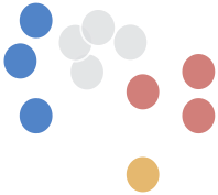
these points come from 2 gaussian distribution.
which point comes from which gaussian?
1
2
3
4-6
7
8
9-12
13
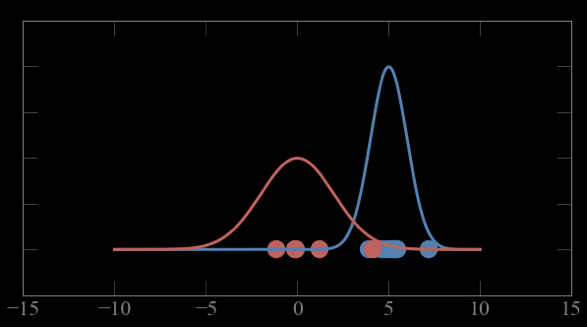
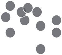
CASE 1:
if i know which point comes from which gaussian
i can solve for the parameters of the gaussian
(e.g. maximizing likelihood)
1
2
3
4-6
7
8
9-12
13
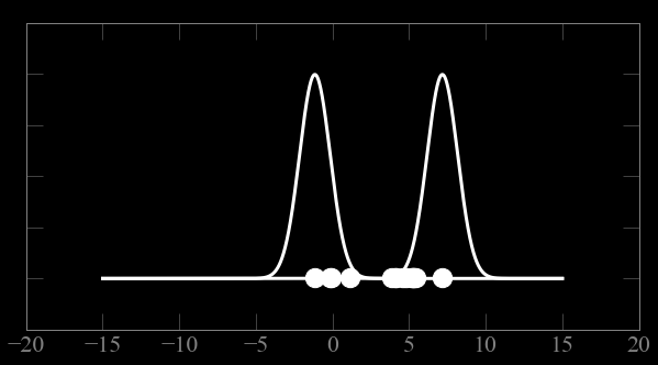
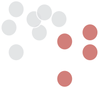
CASE 2:
if i know which the parameters (μ,σ) of the gaussians
i can figure out which gaussian each point is most likely to come from (calculate probability)
1
2
3
4-6
7
8
9-12
13
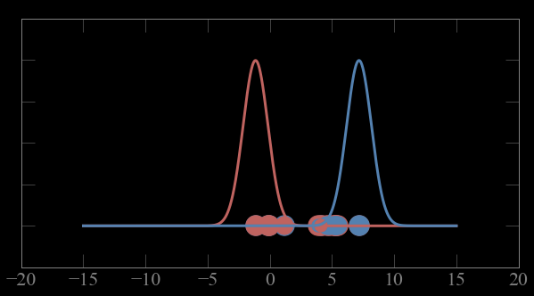
Guess parameters g= (μ,σ) for 2 Gaussian distributions A and B
calculate the probability of each point to belong to A and B
low
Guess parameters g= (μ,σ) for 2 Gaussian distributions A and B
calculate the probability of each point to belong to A and B
Guess parameters g= (μ,σ) for 2 Gaussian distributions A and B
1- calculate the probability p_ji of each point to belong to gaussian j
Bayes theorem: P(A|B) = P(B|A) P(A) / P(B)
Guess parameters g= (μ,σ) for 2 Gaussian distributions A and B
1- calculate the probability p_ji of each point to belong to gaussian j
2a - calculate the weighted mean of the cluster, weighted by the p_ji
Bayes theorem: P(A|B) = P(B|A) P(A) / P(B)
Bayes theorem: P(A|B) = P(B|A) P(A) / P(B)
Guess parameters g= (μ,σ) for 2 Gaussian distributions A and B
1- calculate the probability p_ji of each point to belong to gaussian j
2a - calculate the weighted mean of the cluster, weighted by the p_ji
2b - calculate the weighted sigma of the cluster, weighted by the p_ji
Bayes theorem: P(A|B) = P(B|A) P(A) / P(B)
Alternate expectation and maximization step till convergence
1- calculate the probability p_ji of each point to belong to gaussian j
2a - calculate the weighted mean of the cluster, weighted by the p_ji
2b - calculate the weighted sigma of the cluster, weighted by the p_ji
expectation step
maximization step
}
Last iteration: convergence
Bayes theorem: P(A|B) = P(B|A) P(A) / P(B)
Alternate expectation and maximization step till convergence
1- calculate the probability p_ji of each point to belong to gaussian j
2a - calculate the weighted mean of the cluster, weighted by the p_ji
2b - calculate the weighted sigma of the cluster, weighted by the p_ji
expectation step
maximization step
}
Choose N “centers” guesses (like in K-means)
repeat
Expectation step: Calculate the probability of each distribution given the points

Maximization step: Calculate the new centers and variances as weighted averages of the datapoints, weighted by the probabilities
untill (convergence)
e.g. when gaussian parameters no longer change
Order: #clusters #dimensions #iterations #datapoints #parameters O(KdNp) (>K-means)
based on Bayes theorem
Its non-deterministic: the result depends on the (random) starting point (like K-mean)
It only works where a probability distribution for the data points can be defines (or equivalently a likelihood) (like K-mean)
Must declare the number of clusters and the shape of the pdf upfront (like K-mean)
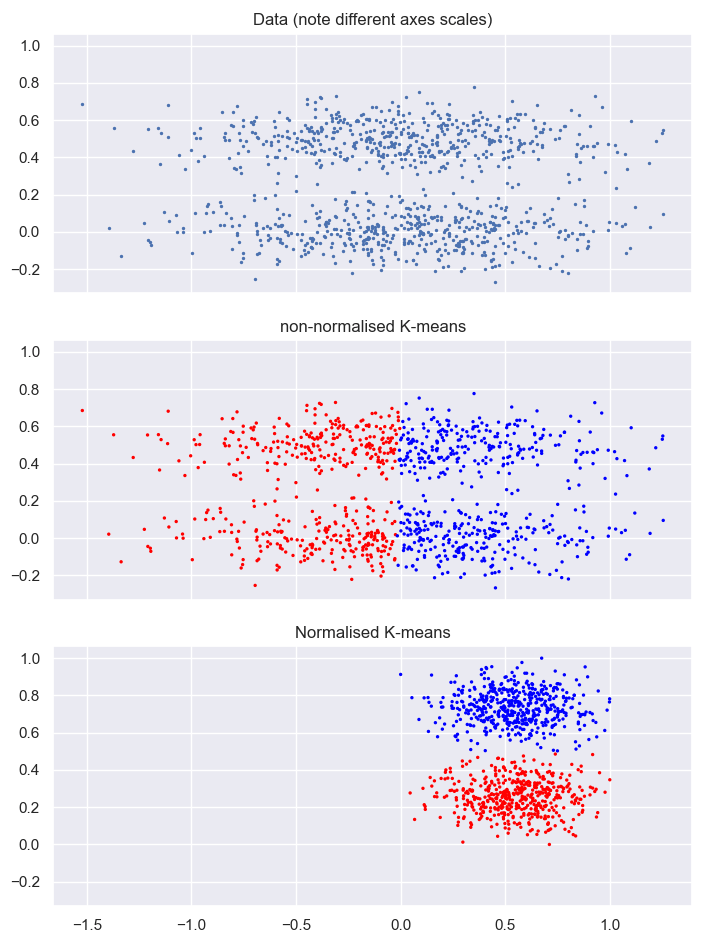
We already saw why we need to scale and how to scale time series when we use the time series values as features.
What happens if we don't scale/wrong scale in clustering??
20 40 50 60 80 100
0.3
0.2
0.1
0.0
assume you have data that looks like this
can you identify grouping?
net pay in $1,000
training time fraction
made up dataset of a company where employees have group-raises evaluated based on their current income and their commitment to self improvement measured by time in training
0.3
0.2
0.1
0.0
assume you have data that looks like this
can you identify grouping?
training time fraction
20 40 50 60 80 100
net pay in $1,000
0.3
0.2
0.1
0.0
is this what you were thinking??
0.3
0.2
0.1
0.0
assume you have data that looks like this
can you identify grouping?
training time fraction
20 40 50 60 80 100
net pay in $1,000
0.3
0.2
0.1
0.0
is this what you were thinking??
range ~100 dominates distance
range ~0.3 becomes insignificant!
0.3
0.2
0.1
0.0
assume you have data that looks like this
can you identify grouping?
training time fraction
0.3
0.2
0.1
0.0
is this what you were thinking??
normalized pay
-1 0 1
1
0
-1
normalized training time fraction
Data that is not correlated appear as a sphere in the Ndimensional feature space
Data can have covariance (and it almost always does!)
ORIGINAL DATA
STANDARDIZED DATA
Generic preprocessing
When standardizing a dataset we take every features and we force them to be the mean=0 standard deviation=1
Generic preprocessing
for each feature: divide by standard deviation and subtract mean
mean of each feature should be 0, standard deviation of each feature should be 1
Time Series Preprocessing
what happens if I standardize a dataset by time stamp??
mean of each feature should be 0, standard deviation of each ROW (time series) should be 1
That way we compare shapes of time series, i.e. trends!
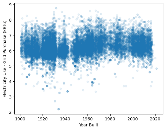
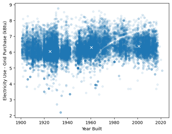
Building dataset: cluster building by time built and electricity used for policy implementation
(add a gap feature to make the dataset more interesting... note the gap around 1940: construction slowed during WWII. our eyes can see three distinct groups.
Can we recover them?
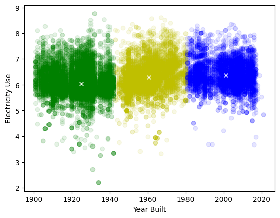
K-means clustering without normalization:
years (order of magnitude 1e3) dominate - horizontal split
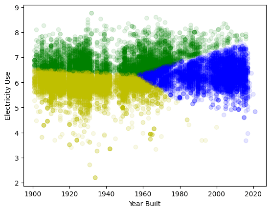
Even on normalized data k-means is not good at finding non spherical patterns and density changes!
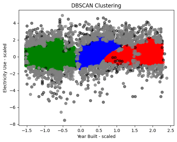
Better option: Density based clustering can recognize density changes and outliers
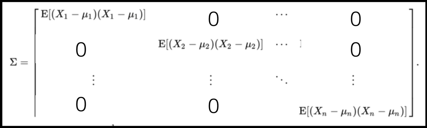
Full On Whitening
: remove covariance by diagonalizing the transforming the data with a matrix that diagonalizes the covariance matrix
axis 1 -> features
axis 0 -> observations
Data can have covariance (and it almost always does!)
Full On Whitening
: remove covariance by diagonalizing the transforming the data with a matrix that diagonalizes the covariance matrix
Full On Whitening
find the matrix W that diagonalized Σ
from zca import ZCA
import numpy as np
X = np.random.random((10000, 15)) # data array
trf = ZCA().fit(X)
X_whitened = trf.transform(X)
X_reconstructed =
trf.inverse_transform(X_whitened)
assert(np.allclose(X, X_reconstructed))
: remove covariance by diagonalizing the transforming the data with a matrix that diagonalizes the covariance matrix
this is at best hard, in some cases impossible even numerically on large datasets
A covariance matrix is diagonal if the data has no correlation
Full On Whitening
: remove covariance by diagonalizing the transforming the data with a matrix that diagonalizes the covariance matrix
Data can have covariance (and it almost always does!)
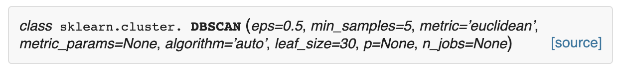
DBSCAN
DBSCAN is one of the most common clustering algorithms and also most cited in scientific literature
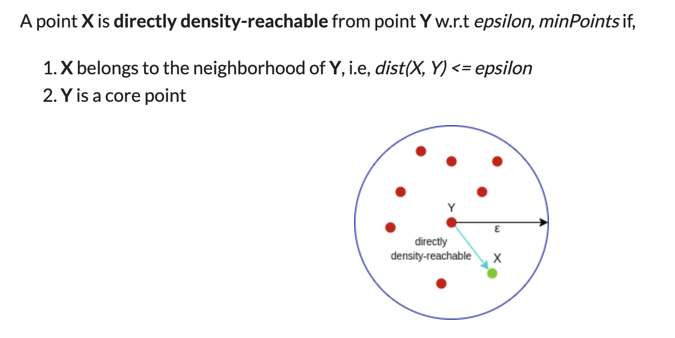
A point p is a core point if at least minPts points are within distance ε (including p).
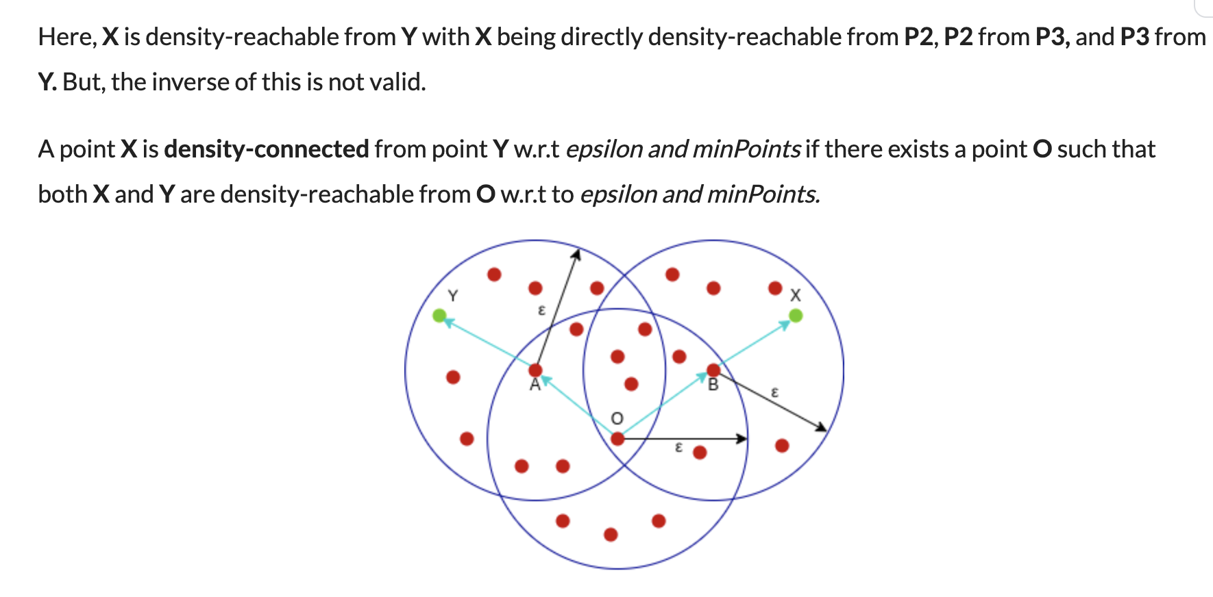
A point q is directly reachable from p if point q is within distance ε from core point p. Reachable from p if there is a path p1, ..., pn with p1 = p and pn = q, where each pi+1 is directly reachable from pi.
All points not reachable from any other point are outliers or noise points.
Density-based spatial clustering of applications with noise
minPts
minimum number of points to form a dense region
maximum distance for points to be considered part of a cluster
ε
Key Hyperparameters:
Density-based spatial clustering of applications with noise
Key Hyperparameters:
minPts
minimum number of points to form a dense region
ε
maximum distance for points to be considered part of a cluster
2 points are considered neighbors if distance between them <= ε
Density-based spatial clustering of applications with noise
minPts
ε
maximum distance for points to be considered part of a cluster
minimum number of points to form a dense region
2 points are considered neighbors if distance between them <= ε
regions with number of points >= minPts are considered dense
Key Hyperparameters:
ε
minPts = 3
slides: Farid Qmar
ε
minPts = 3
slides: Farid Qmar
ε
minPts = 3
ε
slides: Farid Qmar
ε
minPts = 3
directly reachable
slides: Farid Qmar
ε
minPts = 3
core
dense region
slides: Farid Qmar
ε
minPts = 3
slides: Farid Qmar
ε
minPts = 3
directly reachable to
slides: Farid Qmar
ε
minPts = 3
reachable to
slides: Farid Qmar
ε
minPts = 3
slides: Farid Qmar
ε
minPts = 3
reachable
slides: Farid Qmar
ε
minPts = 3
slides: Farid Qmar
ε
minPts = 3
slides: Farid Qmar
ε
minPts = 3
ε
slides: Farid Qmar
ε
minPts = 3
directly reachable
slides: Farid Qmar
ε
minPts = 3
core
dense region
slides: Farid Qmar
ε
minPts = 3
reachable
slides: Farid Qmar
ε
minPts = 3
slides: Farid Qmar
ε
minPts = 3
noise/outliers
slides: Farid Qmar
PROs:
CONs:
ε : minimum distance to join points
min_sample : minimum number of points in a cluster, otherwise they are labeled outliers.
metric : the distance metric
p : float, optional The power of the Minkowski metric
ε : minimum distance to join points
min_sample : minimum number of points in a cluster, otherwise they are labeled outliers.
metric : the distance metric
p : float, optional The power of the Minkowski metric
its extremely sensitive to these parameters!
for each point P count neighbours within minPts: label=C
for each point P ~= C measure distance d to all Cs
        if d<minD: label = DR
for each point P not C and not DR
        if distance d to C or DR > minD: label = outlier
        if distance d to C or DR <= minD: find path to closet C and cluster
Order:
PROs
Deterministic.
Deals with noise and outliers
Can be used with any definition of distance or similarity
PROs
Not entirely deterministic.
Only works in a constant density field
a really good blog post on DBScan
https://www.analyticsvidhya.com/blog/2020/09/how-dbscan-clustering-works/
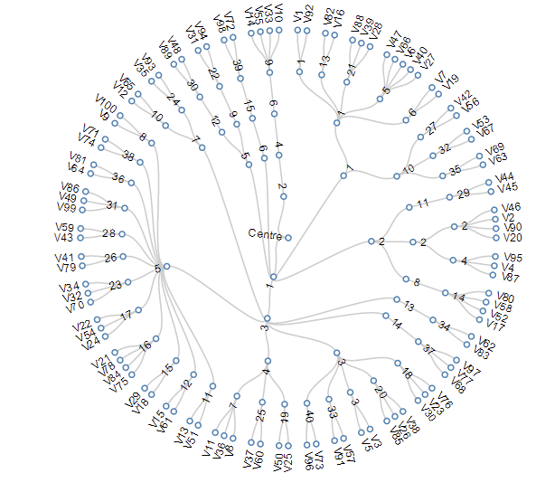
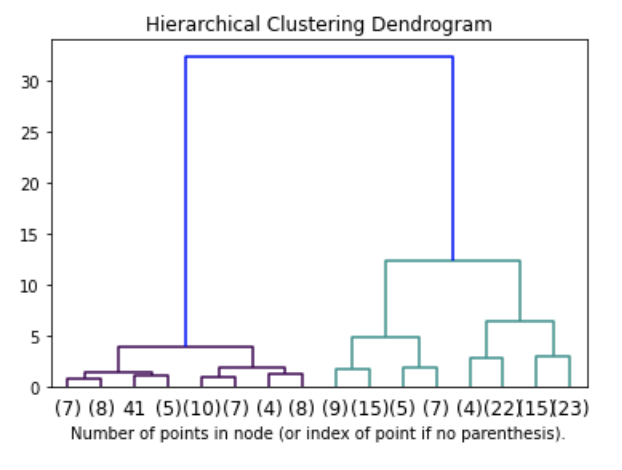
dataset
Cluster Visualization "dendrogram"
distance
it's deterministic!
it's deterministic!
computationally intense because every cluster pair distance has to be calculate
it's deterministic!
computationally intense because every cluster pair distance has to be calculate
it is slow, though it can be optimize:
complexity
compute the distance matrix
each data point is a singleton cluster
repeat
    merge the 2 cluster with minimum distance
    update the distance matrix
untill
    only a single (n) cluster(s) remains
Order:
PROs
It's deterministic
CONs
It's greedy (optimization is done step by step and agglomeration decisions cannot be undone)
It's computationally expensive
distance between a point and a cluster:
single link distance
D(c1,c2) = min(D(xc1, xc2))
distance between a point and a cluster:
single link distance
D(c1,c2) = min(D(xc1, xc2))
complete link distance
D(c1,c2) = max(D(xc1, xc2))
distance between a point and a cluster:
single link distance
D(c1,c2) = min(D(xc1, xc2))
complete link distance
D(c1,c2) = max(D(xc1, xc2))
centroid link distance
D(c1,c2) = mean(D(xc1, xc2))
distance between a point and a cluster:
single link distance
D(c1,c2) = min(D(xc1, xc2))
complete link distance
D(c1,c2) = max(D(xc1, xc2))
centroid link distance
D(c1,c2) = mean(D(xc1, xc2))
Ward distance (global measure)
it is
non-deterministic
(like k-mean)
it is
non-deterministic
(like k-mean)
it is greedy -
just as k-means
two nearby points
may end up in
separate clusters
it is
non-deterministic
(like k-mean)
it is greedy -
just as k-means
two nearby points
may end up in
separate clusters
it is high complexity for
exhaustive search
But can be reduced (~k-means)
or
Calculate clustering criterion for all subgroups, e.g. min intracluster variance
repeat
split the best cluster based on criterion above
untill
each data is in its own singleton cluster
Order: (w K-means procedure)
It's non-deterministic: the result depends on the (random) starting point (like K-mean) unless its exaustive (but that is )
or
It's greedy (optimization is done step by step)
Clustering : unsupervised learning where all features are observed for all datapoints. The goal is to partition the space into maximally homogeneous maximally distinguished groups
clustering is easy, but interpreting results is tricky
Distance : A definition of distance is required to group observations/ partition the space.
Common distances over continuous variables
Common distances over categorical variables:
Whitening
Models assume that the data is not correlated. If your data is correlated the model results may be invalid. And your data always has correlations.
- whiten the data by using the matrix that diagonalizes the covariance matrix. This is ideal but computationally expensive if possible at all
- scale your data so that each feature is mean=0 stdev=2.
Solution:
Partition clustering:
Hard: K-means O(KdN) , needs to decide the number of clusters, non deterministic
simple efficient implementation but the need to select the number of clusters is a significant flaw
Soft: Expectation Maximization O(KdNp) , needs to decide the number of clusters, need to decide a likelihood function (parametric), non deterministic
Hierarchical:
Divisive: Exhaustive ; at least non deterministic
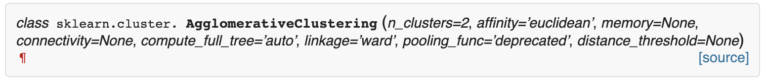
Agglomerative: , deterministic, greedy. Can be run through and explore the best stopping point. Does not require to choose the number of clusters a priori
Density based
DBSCAN: Density based clustering method that can identify outliers, which means it can be used in the presence of noise. Complexity . Most common (cited) clustering method in the natural sciences.
encoding categorical variables:
variables have to be encoded as numbers for computers to understand them. You can encode categorical variables with integers or floating point but you implicitly impart an order. The standard is to one-hot-encode which means creating a binary (True/False) feature (column) for each category of a categorical variables but this increases the feature space and generated covariance.
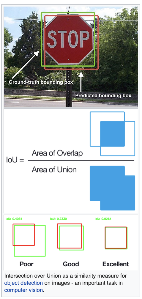
model diagnostics for classifiers: Fraction of True Positives and False Positives are the metrics to evaluate classifiers. Combinations of those numbers include Accuracy (TP/ (TP+FP)), Precision (TP/(TP+FN)), Recall ((TP+TN)/(TP+TN+FP+FN)).
ROC curve: (TP vs FP) is a holistic metric of a model. It can be used to guide the choice of hyperparameters to find the "sweet spot" for your problem
a comprehensive review of clustering methods
Data Clustering: A Review, Jain, Mutry, Flynn 1999
https://www.cs.rutgers.edu/~mlittman/courses/lightai03/jain99data.pdf
a blog post on how to generate and interpret a scipy dendrogram by Jörn Hees
https://joernhees.de/blog/2015/08/26/scipy-hierarchical-clustering-and-dendrogram-tutorial/
https://arxiv.org/html/2412.20582v1
mandatory reading :
Section 1,2,3 all of it
Section 4 and 5.2: pick one method that was not covered in class
Section 5.3-4: pick one method that was not covered in class
By federica bianco
kNN, and DTW


